Chapter 10 Variational Inference
Foreword. This chapter makes heavy use of Blei, Kucukelbir, and McAuliffe (2017) and the following two excellent presentations:
Citations to these three references are generally omitted throughout the text to avoid clutter, and instead we note their importance here.
10.1 Introduction
Let us consider the probabilistic model \(p(\rvx, \rvz)\) with \(\rvz\) and \(\rvx\) being latent and observable variables, respectively. Given an observation \(\rvx\), the corresponding latent variable \(\rvz\) can be inferred using the posterior distribution \[ \begin{align} p(\rvz\mid \rvx) = \frac{p(\rvx, \rvz)}{p(\rvx)}. \end{align} \] For most interesting models, however, the evidence \(p(\rvx) = \int p(\rvx, \rvz)\,d\rvz\) is intractable, and therefore we need to approximate the posterior.
Variational Inference (VI) turns the inference problem into an optimization problem. The first step to VI is to posit a family of approximate densities \(\Q\). We then use optimization techniques to find a member \(q(\rvz; \eet) \in \Q\) that is close to the posterior \(p(\rvz \mid \rvx)\). Generally, closeness is measured using the Kullback-Leibler (KL) divergence \[ \kl \left(q(\rvz; \eet) ~\|~ p(\rvz\mid \rvx)\right), \] however, alternative measures are possible.
Throughout this chapter we will make heavy use of one particular example: Bayesian mixture of Gaussians. In particular, we consider the case of \(K\) mixtures of univariate unit-variance Gaussians. We choose the prior of the \(K\) mean parameters to be a zero-mean Gaussian with hyperparameter \(\sigma^2\), i.e., \(\N \left( 0, \sigma^2 \right)\). Furthermore, we choose the prior on the cluster assignments to be uniform over all \(K\) mixtures. Given a set \(\rvx = \{\rx_i\}_{i=1}^m\) of \(m\) observations, the full hierarichal model is given as
\[\begin{align} \mu_k &\sim \N \left( 0, \sigma^2 \right), \quad &&k = 1, \dots, K, \\ \rvc_i &\sim \tx{Cat}(1/K, \dots, 1/K), \quad &&i = 1, \dots, m, &&\\ \rx_i \mid \rvc_i, \mmu &\sim \N \left( \rvc_i \cdot \mmu, 1 \right), \quad &&i = 1, \dots, m,\end {align}\]
where \(\tx{Cat}\) is the categorical distribution. The evidence of this model can be computed as
\[\begin{align} p(\rvx) = \sum_{\rvc} p(\rvc) \int p(\mmu) \prod_{i=1}^m p (\rx_i \mid \rvc_i, \mmu) \, d\mmu. \end{align}\]
The computational complexity of this integral is \(\O \left( K^m \right)\), and hence intractable for large \(m\).
10.1.1 The Evidence Lower Bound
As discussed before, VI circumvents the inference problem by solving the following optimization problem
\[q^\star(\rvz) = \min_{\eet} \kl \left(q(\rvz; \eet) ~\|~ p(\rvz \mid \rvx)\right).\]
This objective function, however, is not tractable as it requires computing \(\log p (\rvx)\). To see this, we rewrite the KL divergence
\[\kl \left(q(\rvz; \eet) ~\|~ p(\rvz,\mid \rvx)\right) = \E \left[ \log q(\rvz) - \log p(\rvz \mid \rvx) \right],\]
where the expecation is with respect to the variatonal density. Expanding the posterior \(p(\rvz\mid \rvx)\) gives
\[\kl \left(q(\rvz; \eet) ~\|~ p(\rvz \mid \rvx)\right) = \E \left[ \log q (\rvz) - \log p(\rvx, \rvz) + \log p(\rvx) \right],\]
revealing the objective’s dependence on \(\log p(\rvx)\). Since \(\log p(\rvx)\) is a constant with respect to \(\eet\), we can instead optimize the evidence lower bound (ELBO)
\[\begin{align} \tx{ELBO}(q) &= \log p(\rvx) - \kl \left(q(\rvz ; \eet) ~\|~ p(\rvz \mid \rvx)\right) \\ &= \E \left[ \log p(\rvx, \rvz) - \log q(\rvz) \right]. \end{align}\]
Maximizing the ELBO is equivalent to minimizing the KL divergence.
10.1.2 The Mean-Field Variatonal Family
With the ELBO, we just found a tractable variational ojective function. Now, we need to posit a variational family \(\Q\). One practical approach is to let \(\Q\) be within the mean-field variational families, fully-factorizing the variational density \(q(\rvz) = \prod_{j=1}^n q_j(\rvz_j)\). The variational factors \(q_j (\rvz_j)\) are chosen to maximize the ELBO, however, the optimal parametric form of the individual factors has still to be determined. Finding the appropriate form is non-trivial and highly depends on the corresponding random variable.
The mean-field variational family is expressive as it can capture any marginal density of the latent variables, however, it cannot capture correlations between them. Consider the posterior density
\[p(\rvz \mid \rvx) = \N \left( \rvz \mid \bm{0}, \begin{bmatrix} 1 &0.95^2 \\ 0.95^2 &1 \end{bmatrix} \right),\]
where the optimal mean-field variational form is the product of two univariate Gaussians. Figure 10.1 shows the mean-field variational density after maximizing the ELBO (green) and the correct posterior (magenta). The variational factors are by construction decoupled. Furthermore, the marginal variances of the mean-field approximation underrepresent those of the correct posterior. This is a common effect in variational inference due to the structure of the objective function.
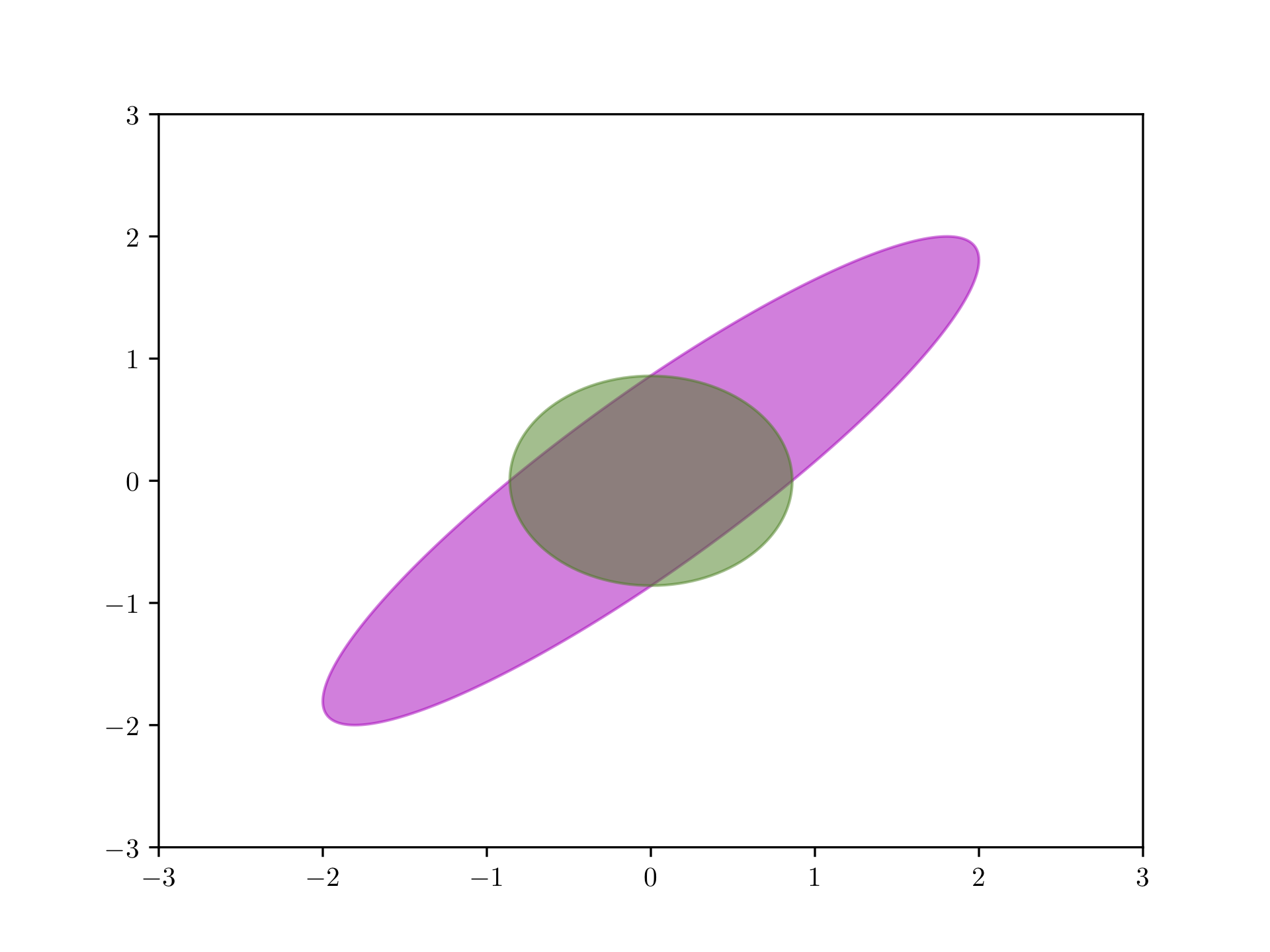
Figure 10.1: Mean field approximation (green) of a Gaussian distribution (magenta).
Let us now come back to our Bayesian mixture of Gaussians example. Following the mean-field recipe, one choice to approximate \(p(\mmu, \rvc \mid \rvx)\) is the following
\[q(\mmu, \rvc) = \prod_{k=1}^K q \left(\mu_k; m_k, s^2_k \right) \prod_{i=1}^m q(\rvc_i; \pps_i),\]
where \(q \left(\mu_k; m_k, s^2_k \right)\) is a normal distribution with mean \(m_k\) and variance \(s^2_k\), and \(q(\rvc_i; \pps_i)\) is a categorical distribution with parameters \(\pps_i\). In fact, it can be shown that these parametric forms for the variational factors are optimal. Is is now left to find the optimal parameters of this mean-field approximation.
10.1.3 Coordinate Ascent Mean-Field Variational Inference
Using the mean-field family and the ELBO, we have casted the approximate inference problem in an optimization problem. One common approach to find the optimal variational parameters is coordinate ascent variational inference (CAVI) (Bishop 2006).
Assume now for a moment that we found the optimal variational factors \(q_l(\rvz_l)\), for all \(l \neq j\). In order to find the remaining optimal factor, \(q_j(\rvz_j)\), we could maximize the ELBO with respect to it. To do so, we will first re-write the ELBO as
\[\begin{align} \tx{ELBO}(q) &= \E \left[ \log p(\rvx, \rvz) - \log q(\rvz) \right] \\ &= \E \left[ \log p(\rvz \mid \rvx) + \log p(\rvx) - \log \prod_{j=1}^n q_j(\rvz_j) \right] \\ &= \log p(\rvx) + \E \left[ \log p(\rvz \mid \rvx) - \sum_{j=1}^n \log q_j(\rvz_j) \right] \\ &= \log p(\rvx) + \E \left[ \log p(\rvz \mid \rvx) \right] + \sum_{j=1}^n \E_{q_j} \left[ q_j(\rvz_j) \right]. \end{align}\]
Hence the optimal \(q_j(\rvz_j)\) given the variational factors \(q_l(\rvz_l)\), for all \(l \neq j\), can be found by solving
\[\begin{align} \argmax_{q_j} \tx{ELBO} &= \argmax_{q_j} \E \left[ p(\rvz_j \mid \rvz_{-j}, \rvx) \right] - \E_{q_j} \left[\log q(\rvz_j) \right] \\ &= \argmax_{q_j} \int_{\rvz_j} q_j(\rvz_j) \left(\E_{q_{-j}} \left[ p(\rvz_j \mid \rvz_{-j}, \rvx) \right] - \log q(\rvz_j) \right) \,d\rvz_j, \end{align}\]
where the notation \(-j\) denotes all indices other than the \(j\)-th. The above equation can be solved by solving
\[ \frac{\partial \tx{ELBO}}{\partial q_j(\rvz_j)} = \E_{q_{-j}} \left[ p(\rvz_j \mid \rvz_{-j}, \rvx) \right] - \log q(\rvz_j) -1 = 0.\]
Hence,
\[ \begin{align} \tag{10.1} q(\rvz_j) \propto \exp \left( \E_{q_{-j}} \left[ p(\rvz_j \mid \rvz_{-j}, \rvx) \right] \right), \end{align} \]
or equivalently
\[ q(\rvz_j) \propto \exp \left( \E_{q_{-j}} \left[ p(\rvz_j, \rvz_{-j}, \rvx) \right] \right).\]
The idea of CAVI is to iterate through the variational factors, updating one factor at a time using Equation (10.1). Every update will improve the ELBO until CAVI eventually converges to a local maximum. CAVI is closely related to Gibbs sampling (Geman and Geman 1984), a popular Markov chain Monte Carlo method for approximate inference.
Let us return to our example. We now state the variational updates and refer to Section 3 of Blei, Kucukelbir, and McAuliffe (2017) for the derivations. The variational update for the \(i\)-th cluster assignment is
\[\psi_{ik} \propto \exp \left(m_k \rx_i - \left(s_k^2 + m_k^2 \right) \right).\]
The variational updates for the mean and variance of \(q \left(\mu_k; m_k, s^2_k \right)\) are
\[m_k = \frac{\sum_{i=1}^m \psi_{ik} \rx_i}{\sigma^{-2} + \sum_{i=1}^m \psi_{ik}},\]
and
\[s_k^2 = \frac{1}{\sigma^{-2} + \sum_{i=1}^m \psi_{ik}}.\]
We now run the CAVI algorithm on a dataset of size \(m = 1000\) for 50 iterations using five different initializations. Figure 10.2 shows the increasing behavior of the ELBO. Different initializations lead to different converge behaviors, however, all runs seem to have converged after roughly 30 iterators. In this simulation, we do not compute the ELBO exactly but rather approximate it using 100 Monte Carlo samples, justifying the up-and-down-jumping behavior that is present after roughly 20 iterations.
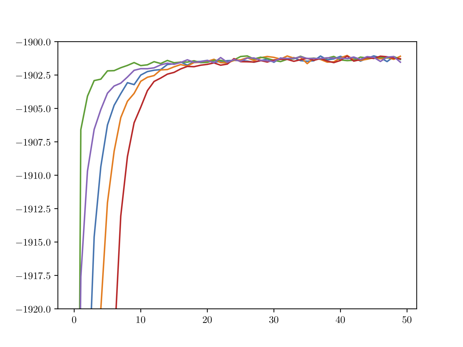
Figure 10.2: (Approximated) ELBO over number of CAVI iterations for Bayesian mixture of Gaussians; runs over five different initializations.
10.2 Variational Inference with Exponential Families
We just worked out the general CAVI algorithm and demonstrated it on our Bayesian mixture of Gaussians example with each coordinate update being available in closed form. The property that allowed to find these closed form updates was that each complete conditional \(p(\rvz_j \mid \rvz_{-j}, \rvx)\) of the model is in the exponential family. As it turns out, there are many models that share this property with the Bayessian mixture of Gaussians; to name a few:
- Matrix factorization models
- Linear regression
- Hierarichal mixture of experts
Working within this family of models lets us derive a special form of the CAVI algorithm and lets us scale up VI to large datasets.
10.2.1 Complete Conditionals in the Exponential Family
We say that a complete conmditional \(p(\rvz_j \mid \rvx, \rvz_{-j})\) is in the exponetial family if the probabilty density function can be written as
\[p(\rvz_j \mid \rvx, \rvz_{-j}) = \sfh_j(\rvz_j) \exp \left( \sfk_j(\rvx, \rvz_{-j}) \rvz_j - \sfa_j(\sfk_j(\rvx, \rvz_{-j})) \right),\]
for some \(\sfh_j\), \(\sfk_j\), and \(\sfa_j\). This assumption simplifies the cooardinate update of Equation (10.1)
\[ q(\rvz_j) \propto \sfh(\rvz_j) \exp \left( \E_{q_{-j}} \left[ \sfk(\rvx, \rvz_{-j}) \right] \rvz_j - \E_{q_{-j}} \left[\sfa(\sfk_j(\rvx, \rvz_{-j}))\right]\right),\]
revealing the parametric form of the optimal variational factors, i.e.,
\[ q(\rvz_j; \eet_j) = \sfh(\rvz_j) \exp \left( \eet_j \rvz_j - \sfa(\eet_j)\right).\]
When we update the variational factors, we can just update their parameters as
\[ \eet_j \leftarrow \E_{q_{-j}} \left[ \sfk_j(\rvx, \rvz_{-j}) \right]. \]
10.2.2 Conditional Conjugacy
In this section, we discuss a special class of models: conditionally conjugate models. In conditionally conjugate models, the latent variables can be separated into two classes: local latent variables \(\rvzl\) and global latent variables \(\rvzg\). The global latent variables potentially govern all of the data, whereas the \(i\)-th local latent variable only applies to the \(i\)-th datapoint \(\rvx_i\). The joint density can then be written as
\[p(\rvx, \rvzl, \rvzg) = p(\rvzg) \prod_{i=1}^m p(\rvx_i, \rvzl_i \mid \rvzg).\]
In our example, the \(K\) mean parameters are global latent variables and the \(m\) cluster assignments are local latent variables.
We now look at a subset of all conditionally conjugate models. In particular, we assume that each complete conditional is in the exponential family, i.e.,
\[p(\rvzl_i \mid \rvx, \rvzg) = \sfhl_i(\rvzl_i) \exp \left( \sfkl_i(\rvx_i, \rvzg) \rvzl_i - \sfal_i(\sfkl_i(\rvx_i, \rvzg)) \right),\]
and
\[p(\rvzg \mid \rvx, \rvzl) = \sfhg(\rvzg) \exp \left( \sfkg(\rvx, \rvzl) \rvzg - \sfag(\sfkg(\rvx, \rvzl)) \right).\]
It can be shown (Bernardo and Smith 2009) that in this case, we have
\[ \sfkg(\rvx, \rvzl) = \aal + \sum_{i=1}^m \sft_i(\rvx_i, \rvzl_i), \]
where \(\aal\) is a hyperparamter and \(\sft_i\) are sufficient statistics for \((\rvx_i, \rvzl_i)\). Using the mean-field family, we choose each factor to be in the same family as the model’s complete conditional, i.e.,
\[q(\rvzl_i \mid \rvx, \rvzg) = \sfhl_i(\rvzl_i) \exp(\gga_i \rvzl_i - \sfal_i(\gga_i)),\]
and
\[q(\rvzg \mid \rvx, \rvzl) = \sfhg(\rvzg) \exp(\tta \rvzg - \sfag(\tta)),\]
where \(\gga_i\) and \(\tta\) are the variational parameters. Given the specific form of \(\sfkg\) the updates of the variational parameters are
\[ \gga_i \leftarrow \E_{q(\rvzg)}[\sfkl_i(\rvx_i, \rvzg)], \]
and
\[ \tta \leftarrow \aal + \sum_{i=1}^m \E_{q(\rvzl_i)} \left[ \sft(\rvx_i, \rvz_i) \right].\]
10.2.3 Stochastic Variational Inference
Let’s sum up what has happened so far. We have derived the ELBO, a tractable objective function for VI. We then introduced the mean-field variational family to model the approximate posterior distribution. Furthermore, we derived CAVI, an algorithm for finding the optimal variational paramters when using the mean-field variational family. Using models with their complete conditionals in the exponential family, we found that the optimal updates for CAVI are simple to derive. Using conditionally conjugate models, these updates became even simpler. It is left to treat one major caveat: large data.
Let us assume we are in the setting of conditionally conjugate models with complete conditionals in the exponential family. The idea of stochastic variational inference (SVI) (Matthew D. Hoffman et al. 2013) is that we just update some of the local paramters in each iteration. Additionally, instead of using CAVI, SVI updates the parameters using a method that combines natural gradients (Amari 1998) and stochastic optimization (Robbins and Monro 1951). In this section, we assume that the reader is familiar with stochastic gradient based optimization methods, e.g. stochastic gradient ascent (SGD). In our framework, the natural gradient of the ELBO can be computed as
\[ \nabla_\eet^{\tx{nat}} \tx{ELBO} = \aal + \sum_{i=1}^m \E_{q(\rvzl_i)} \left[ \sft(\rvx_i, \rvz_i) \right] - \eet .\]
We can easily construct an unbiased estimate of the natural gradient by first sampling \(j \sim \U\{1, \dots, n\}\), where \(\U\) is the uniform distribution, and then computing
\[ \hat{\nabla}_\eet^{\tx{nat}} \tx{ELBO} = \aal + m \E_{q(\rvzl_j)} \left[ \sft(\rvx_j, \rvz_j) \right] - \eet .\]
Note that the estimate is very cheap as it only dependens on one data point. One iteration of the SVI algorithm, using SGD, then behaves as follows:
- Sample \(j \sim \U\{1, \dots, n\}\)
- Update the \(j\)-th local paramters as \(\gga_j \leftarrow \E_{q(\rvzg)}[\sfkl_j(\rvx_j, \rvzg)]\)
- Update the global parameters as \(\eet \leftarrow \eet + \rho \left(\aal + m \E_{q(\rvzl_j)} \left[ \sft(\rvx_j, \rvz_j) \right] - \eet \right)\)
10.3 Modern Variational Inference
It is time to shift gears and to cut out some assumptions. We want to look at variational inference for any model not just conditionally conjugate models with each complete conditional in the exponential family. To see the importance of this, consider the example of Bayesian logistic regression. Our data for this example is pairs \((\rx_i, \ry_i)\) where \(\rx_i \in \R\) is a covariate and \(\ry_i \in \{0, 1\}\) is a binary label. Let \(\rz\) be the regression coefficient with prior \(p(\rz) = \N(0, 1)\). Bayesian logistic regression than posits the following generative process of labels
\[ \ry_i \mid \rx_i, \rz \sim \tx{Bernoulli}(\sigma(\rx_i \rz)), \]
where \(\sigma\) is the sigmoid function. Using the variational family \(q \left(\rz ; \mu, \sigma^2 \right) = \N \left(\mu, \sigma^2 \right)\) the ELBO can be computed as
\[ \begin{align} \tx{ELBO} &= \E_q \left[ \log p(\rz) - \log q \left(\rz; \mu, \sigma^2 \right) + \sum_{i=1}^m \log p(\ry_i \mid \rx_i, \rz) \right] \\ &= -\frac{1}{2} \left(\mu^2 + \sigma^2 \right) + \frac{1}{2} \log \sigma^2 + \sum_{i=1}^m \ry_i \rx_i \mu - \sum_{i=1}^m \E_q \left[ \log (1 + \exp(\rx_i \rz))\right],\end{align}\]
where we cannot compute the last expectation analytically, and hence we are stuck. To this end, we briefly discuss three ideas: the score gradient, the reparameterization trick, and amortized variational inference. For a more extensive discussion on modern variational inference, we refer the reader to the following presentation.
10.3.1 The Score Gradient
The idea of the score gradient is that instead of solving the expectations in the ELBO analytically, we write the gradient of the ELBO itself as an expectation, i.e.,
\[ \nabla_\eet \tx{ELBO} = \E_{q(\rvz; \eet)} \left[ \nabla_\eet \log q(\rvz; \eet) \left( \log p(\rvx, \rvz) - \log q(\rvz; \eet) \right) \right].\]
We can then jointly update all variational parameters using the following algorithm
- Take \(K\) samples from the variational distribution: \(\rvz_k \sim q(\rvz; \eet_t)\)
- Calculate the noisy score gradient: \(\hat{g}_t = \frac{1}{K} \sum_{k=1}^K \nabla_\eet \log q(\rvz_k; \eet_t) \left( \log p(\rvx, \rvz_k) - \log q(\rvz_k; \eet_t) \right)\)
- Update the variational paramters as \(\eet_{t+1} = \eet_{t} + \rho \hat{g}_t\)
For this approach, we do not need any model-specific analysis. One of the problems with this approach, however, is that though the gradient estimate is unbiased it might suffer from very high variance. Methods to control the variance have been developed, some examples are: Rao-Blackwellization, control variates, importance sampling, etc.
10.3.2 The Reparameterization Trick
A lower variance alternative to the score gradient can be achieved using the reparamterization trick. For this to work, we need to express the variational distribution using a transformation, i.e.,
\[ \begin{align} \pph &\sim s(\pph) \\ \rvz &= \sfr(\pph; \eet) \implies \rvz \sim q(\rvz; \eet) \end{align}.\]
As an example, consider the normal distribution with mean \(\mu\) and variance \(\sigma^2\). Using the auxiliary variable \(\phi \sim \N(0, 1)\), we can sample from \(\rz\) using the transformation \(\rz = \phi \sigma + \mu\).
Furthermore, we need to assume that both \(\log p(\rvx, \rvz)\) and \(\log q(\rvz; \eet)\) are differentiable with respect to the latent variables \(\rvz\). The reparameterization gradient can then be computed as
\[ \nabla_\eet \tx{ELBO} = \E_{\sfr(\pph)} \left[ \nabla_\rvz \left( \log p(\rvx, \rvz) - \log q(\rvz; \eet) \right) \nabla_\eet \sfr(\pph, \eet) \right]. \]
It turns out that the reparameterization gradient has lower variance than the reparameterization gradient, however, it comes at the cost of making assumptions on the model and the variational distribution.
10.3.3 Amortized Variational Inference
The last thing we discuss is amortized variational inference (AVI). AVI takes advantage of the recent breakthroughs of deep learning and models the variational distributions for all paramters using a recognition network. The recognition newtork is a neural network that maps the data \(\rvx\) to the variational paramters \(\eet\). Combining the ideas of the reparameterization trick and AVI led to the development of one of the most widely used generative models: the Variational Auto-Encoder (Kingma and Welling 2014; Rezende, Mohamed, and Wierstra 2014).