Chapter 3 Hamiltonian Monte Carlo
Instead of the random walk, the Hamiltonian (or Hybrid) Monte Carlo(HMC) employs the Hamiltonian dynamics in the Metropolis algorithm and explores the target distribution rapidly. This chapter will firstly offer a delicate example of Hamiltonian dynamics in physics as an appetizer. Then the technical details and fundamental properties of the Hamiltonian dynamics will be discussed before getting into HMC algorithm. Several examples will be offered along to make it easy to follow.
3.1 Hamiltonian Dynamic Example in Physics
In physics, simple harmonic oscillator, bouncing ball and the soap slithering are all realizations of Hamiltonian dynamics. Radford M. Neal (2012) visualized the dynamics as of a frictionless puck sliding over a surface of varying height. In this section, the frictionless puck will slide over a miniature half-pipe ramp, which is a symmetric U-shaped skateboard ramp with a flat bottom in the middle. The total energy, or the Hamiltonian, of the puck \(\Ha\) can be classified into the potential energy \(\Ua\) and the kinetic energy \(\Ka\) such that
\[ \Ha (p,q) = \Ua (q) + \Ka (p) \]
The potential energy \(\Ua(q)\) is proportional to the position (\(q\)), for example, the height of the puck in this case.
The kinetic energy is explicitly defined in physics by \(\Ka(p) = \frac{p^2}{2m}\), where \(p\) is the momentum and \(m\) is the mass of the puck.
Note that the momentum is the product of the velocity and the mass of the momentum such that the faster the puck moves, the more momentum (and hence the kinetic energy) it possesses.
One characteristic of the Hamiltonian dynamics is energy conservation: no energy gain/loss of the puck such that \(\Ha(p,q)\) will remain constant over time. On the other hand, the allocation of the energy into \(\Ua(q)\) and \(\Ka(p)\) may vary with the movement of the puck. A few representative scenarios will spotlight such energy transfer and interpret the duality of the potential energy and the kinetic energy.
Moving along the flat bottom, the puck will not experience any energy transfer between potential energy and kinetic energy as the momentum and the height will remain the same.
When the puck at \((p_0, q_0)\) starts to climb the rising slope on one side, it’s going to mountaineer at a decreasing velocity. As it gets slower and higher, more kinetic energy \(\Ka\) is converted to the potential energy \(\Ua\).
When the velocity dwindles to zero so that \(\Ka = 0\), the puck achieves its highest point and set out to slide back down with increasing velocity. The energy transfers back from \(\Ua\) to \(\Ka\).
When the puck returns to the state \((p_0, q_0)\), it continues to move mildly on the flat bottom and then perform similar motions on the other side. With the invariant Hamiltonian over time, the highest point that the puck could achieve on either side in each round trip will remain the same.
In later discussion, the height and the momentum are colloquially referred to as the position variable (\(x\)) and momentum variable (\(v\)) respectively.
3.2 Hamiltonian Dynamics
The \(N\)-dimensional Hamiltonian system consists of \(N\) particles deferring to Hamiltonian dynamics. The state of the system at time \(t\) can be described by (\(\xx_t, \vv_t\)) with position variables \(\xx = (\rv x N)\) and momentum variables \(\vv = (\rv v N )\).
The \(2N\)-dimensional position-momentum phase space is the collection of all possibles states of the system. The phase space trajectory \(\GGa_t = (\xx_t, \vv_t)\) traces out the evolution of the \(N\) particles over time.
3.2.1 Hamiltonian’s Equations
The Hamiltonian function \(\Ha(\xx, \vv, t)\) can be described by the set of differential equations, also known as the Hamilton’s equations:
\[ \begin{equation} \der tx_i(t) = + \del{v_i} \Ha(\xx_t, \vv_t, t), \qquad \der t v_i(t) = - \del{x_i} \Ha(\xx_t,\vv_t,t) \tag{3.1} \end{equation} \] Note that the Hamiltonian itself is not a function of time, however, the \(\Ha(\xx, \vv, t)\) is used to pinpoint the evolution of the position \(\xx_t\) and momentum \(\vv_t\) over time.
The Hamilton’s equations are deterministic, i.e. if the initial state \((\xx_0, \vv_0)\) is known, then the dynamics of the system can be simulated from the Hamiltonian equations. Let \(\IH_t: \mathbb R^{2N} \to \mathbb R^{2N}\) denote the deterministic function that maps the the initial state \(\GGa_0\) at time \(t = 0\) to the solution of the Hamilton’s equations \(\GGa_t\) at time \(t\): \[ \GGa_t = \IH_t(\GGa_0) = \IH(\GGa_0, t). \]
3.2.2 The Hamiltonian - Boltzmann Distribution
Finite Hamiltonian systems are generally not ergodic by virtue of the invariant Hamiltonian. However, excellent physical prediction can be obtained via the stationary distribution \(\paug\). The Boltzmann Distribution defines the joint distribution of \(\GGa = (\xx, \vv)\) as follows. \[ \begin{equation} \paug(\GGa) \propto \exp\left\{-\frac{\Ha(\GGa)}{\kbt}\right\} = \exp\left\{-\frac{\Ua(\xx)}{\kbt}\right\}\exp\left\{-\frac{\Ka(\vv)}{\kbt}\right\}. \tag{3.2} \end{equation} \]
where \(k_{\tx{B}}\) is the Boltzmann constant and \(T\) is the system temperature. For simplicity, \(\kbt\) can be viewed as a constant term.
Further, the kinetic energy of the \(N\) particles is given by \[ \begin{equation} \Ka(\vv_t) = \frac{\vv_t^T\diag(\mm)^{-1}\vv_t}{2} \tag{3.3} \end{equation} \] where \(\diag(\mm)\) is the diagonal mass matrix, often a scalar multiple of the identity matrix. It’s apparent that \(\Ka(\vv_t)\) corresponds to the log probability density of a Gaussian distribution.
This joint distribution (3.2) announces that \(\xx\) and \(\vv\) have independent Boltzmann distributions with energy functions \(\Ua(\xx)\) and \(\Ka(\vv)\) respectively. From the perspective of statistics, it’s equivalent to the following:
\[ \xx, \vv \sim \paug(\xx, \vv) \iff \xx \sim p(\xx) \propto \rho(\xx) \quad \amalg \quad \vv \sim \N(\bz, \diag(\mm)) \] Here \(\rho(\xx)\) is introduced to incorporate the Bayesian inference \(p(\tth \mid \yy) \propto \rho(\tth) = \mathcal L(\tth \mid \yy) \times \pi(\tth)\).
For \(\kbt = 1\), the joint probability \(p(\xx,\vv) \propto \exp\{-\Ha(\xx,\vv)\}\) leads to \[ \begin{equation} \Ha(\xx, \vv) = -\log \rho(\xx) + \tfrac 1 2 \sum_{i=1}^N m_i^{-1} v_i^2 \tag{3.4} \end{equation} \]
3.2.3 Properties of Hamiltonian Dynamics
Before getting into the HMC, we’ll discuss the three fundamental properties of the Hamiltonian dynamics granting the feasible and efficient HMC proposal.
Time Reversibility The simple intuition behind the reversibility is that the initial state can be traced back from some time \(t\). Mathematically, this is accomplished by negating the time derivative in Hamilton’s equations. This property acknowledges \(\IH\) is a one-to-one mapping with the corresponding inverse mapping \(\IH_t^{-1}: \mathbb R^{2N} \to \mathbb R^{2N}\) such that \(\GGa_0 = \IH_t^{-1}(\GGa_t)\).
The time reversibility will not be literally translated in programming HMC but it guarantees the convergence of HMC in the sense that a reversible Markov chain transitions will be generated.
Besides, in the light of the quadratic form of the kinetic energy \(\Ka(v) = \frac{v^2}{m}\), negating the momentum \(v\) can also carry it out. It can be confirmed in the frictionless puck example. At a fixed spot on the rising slope, the position of the puck and hence its potential energy is fixed. Let \(t\) denote the time when the puck achieves the highest point on one of the concave ramps, and \(t-s\) be the time when the puck pass this point during its climbing, then it will slide back down to this point at time \(t+s\). The allocation of its energy is the same at \(t-s\) and \(t+s\), while the direction of the velocity and therefore the momentum are opposite. This is sometimes referred to as bouncing and provides an efficient alternative when constrained parameters are involved(See Section 3.3.2.1).
Energy Conservation The Noether’s theorem states that \(\Ha(\xx, \vv)\) does not depend on \(t\) if the temperature of the system \(T\) is constant. This can also be proved mathematically from the equation (3.1). \[ \frac{\partial\Ha}{\partial t} = \frac{\partial\Ha}{\partial \xx_i} \frac{\mathrm{d}\xx_i}{\mathrm{dt}} + \frac{\partial\Ha}{\partial \vv_i} \frac{\mathrm{d}\vv_i}{\mathrm{dt}} = \frac{\partial\Ha}{\partial \xx_i} \frac{\partial\Ha}{\partial \vv_i}+ \frac{\partial\Ha}{\partial \vv_i}(-\frac{\partial\Ha}{\partial \xx_i}) = 0 \]
This conservation property makes \(\Ha(\xx, \vv)\) constant over the phase space trajectory \(\GGa_t = (\xx_t, \vv_t)\), as declared in the frictionless puck example. It will be seen later that, theoretically, this invariant \(\Ha\) makes the acceptance rate of HMC algorithm to be 1.
Volume preservation The phase space volume occupied by \(\GGa_t\) will be preserved over time. This is a result from the Liouville’s theorem where the density of the \(N\) particles in the phase space are invariant over time.
Mathematically, this property deciphers that the change of variables \(\GGa_0 \to \GGa_t\) has a Jacobian of 1(the derivation can be found in this compact lecture note.):
\[ \left| \frac{\partial \GGa_t}{\partial \GGa_0} \right|= 1 \]
Together with the first two properties, it signifies that \(\paug(\xx,\vv)\) is invariant to the Hamiltonian change-of-variables \(\GGa_t = \IH(\GGa_0,t)\); that is, if \(\paug(\GGa_0) \sim \exp\{\Ha(\xx_0, \vv_0)\}\) then \[ \begin{aligned}[t] \textstyle \paug(\GGa_t) &= \paug\left(\IH_t^{-1}(\GGa_t)\right)\times \left| \frac{\partial \GGa_t}{\partial \GGa_0} \right|\\ & \sim \exp\{\Ha(\xx_0, \vv_0)\} \times 1\\ & = \exp\{\Ha(\xx_t, \vv_t)\} \end{aligned} \]
3.3 Hamiltonian Monte Carlo
This section will streamline HMC algorithm step by step. The goal is to sample the parameter of interest from the target distribution, i.e the position variable \(\xx \sim p(\xx)\). To embody the concept of the Hamiltonian dynamics, the auxiliary momentum variable \(\vv\) of the same dimension will be introduced.
Given the current state \(\GGa_\curr = (\xx_\curr, \vv_\curr)\), the HMC iteration will proceed as follows:
- Generate the momentum variable: \(\vv_0 \sim \N(\bz, \diag(\mm))\)
- Propose the trajectory: \(\GGa_\prop = \mathfrak P\{\GGa_0, t\} = \GGa_t\), where \(\GGa_0 = (\xx_\curr, \vv_0)\)
- Metropolis acceptance step
Note that the first iteration may start with \(\xx_\curr\) and introduce the auxiliary momentum with the first step. As with other MCMC algorithms, the above iterations will be repeated until it converges.
3.3.1 Step 1: Momentum Distribution
The random draw from the momentum distribution \(\vv_0 \sim \N(\bz, \diag(\mm))\) is actually a Gibbs update since \(\xx\) and \(\vv\) are independent (See Section 3.2.2). The mass matrix \(\diag(\mm)\) is the algorithm parameter to be tuned in Section 3.5.1.
On the other hand, any Gibbs update can be viewed as a Metropolis update such that the acceptance probability of this step is \[ \alpha_1 = \underbrace{\frac{p(\xx_\curr, \vv_0)/p(\vv_0 \mid \xx_\curr)}{p(\xx_\curr, \vv_\curr)/p(\vv_\curr \mid \xx_\curr)}}_{p(\xx, \vv)/p(\vv \mid \xx) = p(\xx)} = \frac{p(\xx_\curr)}{p(\xx_\curr)} = 1 \]
That being said, this step will be admitted for sure, where no acceptance step is needed in practice. With the updated momentum, the initial trajectory proceeding of the next step is \(\GGa_0 = (\xx_\curr, \vv_0)\).
3.3.2 Step 2: \(L\)-Step Leap-Frog Integrator
From equations (3.1) and (3.4), \(\GGa_t = \mathfrak P\{\GGa_0, t\}\) is therefore given by \[ \der t x_i(t) = m_i^{-1} v_i(t), \qquad \der t v_i(t) = \del{x_i} \log \rho(\xx). \]
However, the above ordinary differential equations(ODEs) can’t be solved analytically on the phase space except several simple cases. The leap-frog integration is able to approximate the differential equations by discretizing time with small step size \(\eps = t/L\), where (\(L, \eps\)) are parameters of the algorithm to be tuned (See Section 3.5.2). Then, for each one of the \(L\) steps, the evolution kernel \(\hat \IH_\eps\) is given by
\[ \begin{equation} \begin{split} \tilde \vv_\eps & = \vv + (\eps/2) \cdot \nabla \log \rho(\xx) \\ \tilde \xx & = \xx + \eps \cdot \tilde \vv_\eps/\mm \\ \tilde \vv & = \tilde \vv_\eps + (\eps/2) \cdot \nabla \log \rho(\tilde \xx) \end{split} \tag{3.5} \end{equation} \] where \(\nabla \log\rho(\xx)=\langle \del {x_1} \log\rho(\xx), \dots, \del {x_N} \log\rho(\xx) \rangle\) is the gradient vector. The HMC proposal is obtained by repeating the above procedure \(\hat \IH_\eps\) for \(L\) times, denoted by \[\GGa_t = \IH_t{\GGa_0} = \hat \IH_\eps^{L}\{\GGa_0\} = \underbrace{\hat \IH_\eps \circ \cdots \circ \hat \IH_\eps}_{\times L} \{\GGa_0\}.\]
The leap-frog integrator is a second-order symplectic integrators that will guarantee the generated trajectories to comply with the three properties discussed in Section 3.2.3. In particular, the preserved volume in the phase space allows the proposals meander around the exact trajectories. In contrast, Radford M. Neal (2012) applied the Euler method, which doesn’t conform to this property, to approximate the dynamics and a trajectory that diverges to infinity was proposed.
3.3.2.1 Constrained Parameters
At the end of each evolution kernel \(\hat \IH_\eps\), whether the posterior probability is positive will be checked to make sure the HMC proposal is not out of range at this step. Failing to pass this routine check indicates some of the parameters are out of the boundaries. If this happens, the blunt option is to reject the proposal to terminate this iteration immediately and set up the next iteration with \(\xx_\curr\).
Transformation of parameters to unconstrained scales is another option. For example, log transformation (\(\mathbb R^{+} \to \mathbb R\)) and logit transformation (\((0,1) \to \mathbb R\)) are commonly used. In this case, the posterior probability and its gradient after the change of variable must be figured out.
Alternatively, the bouncing characteristic in Section 3.2.3 can be quoted. Changing the sign of the momentum will reject this evolution kernel \(\hat \IH_\eps\) and return to the updates in the previous kernel. Rejecting this single sub-step is typically more efficient than rejecting the whole iteration.
3.3.3 Step 3: Metropolis acceptance procedure
The HMC proposal \(\GGa_\prop\) is accepted with the probability \[ \alpha=\min\left\{1, \frac{p(\GGa_\prop)} {p(\GGa_0)}\right\} = \min\left\{1, \frac{\exp(\Ha(\GGa_0))} {\exp(\Ha(\GGa_\prop))}\right\} \] Theoretically, the energy conservation discussed in Section 3.2.3 states that \(\Ha(\GGa_t) = \Ha(\GGa_0)\). Therefore, if the ODEs can be solved analytically such that \(p(\GGa_0) = p(\GGa_\prop)\) and the proposal will always be accepted.
The HMC proposals generated numerically are not deterministic, while Hamilton’s equations are deterministic (See Section 3.2.1). Though the leap-frog integrator is highly accurate, the numerical approximation will bias the proposed trajectory such that the Hamiltonian will not be exactly conservative. Besides, the leap-frog approximation will not be perfectly reversible in practice due to rounding calculation.
In this sense, the \(\Ha(\GGa_t)\) will depart away from \(\Ha(\GGa_0)\) and the acceptance rate would not achieve 1. By treating the proposal as a stochastic one, the Metropolis acceptance step is embraced to compensate for this deviation. However, this deviation is fairly small and the resulting acceptance probability is relatively high, which makes HMC efficient.
3.3.4 Example: Visualization of the HMC Proposal
Figure 3.13 visualizes the dynamics of an HMC proposal for the standard normal with the energy defined by \(\Ha(x,v) = \Ua(x)+\Ka(v)=\frac{x^2}{2}+\frac{v^2}{m}\) such that
\[ x \sim \N(0,1) \quad v \sim \N(0,m) \]
Given the initial state \(\GGa_\curr = (x_\curr, v_\curr)\), the HMC proposal is specified as follows:
Generate a Gibbs proposal \(v_0 \sim \N(0,m)\) such that \(\GGa_0 =(x_0, v_0)=(x_\curr, v_0)\).
In practice the evolution kernel \(\hat \IH_t\) can rarely be computed exactly, where the leap-frog approximation will be utilized in place. However, the evolution kernel \(\hat \IH_t\) can be solved explicitly for this model and the analytic solution is
\[ \begin{aligned} x_t & = x_0 \cos(\lambda t) - \lambda v_0 \sin(\lambda t) \\ v_t & = v_0 \cos(\lambda t) + \lambda^{-1} x_0 \sin(\lambda t), \qquad \lambda = m^{-1/2}. \end{aligned} \] As mentioned in Section 3.3.2, the availability of the analytic solution empowers the HMC proposal to be accepted for sure.
Figure 3.1: Visualization wiht slider of parameters:(a)Topleft: density plot of prposed energy level; (b) Topright: contour plot: each ellipse is a level set of postion and momentum variables with a fixed energy level; (c)Bottom: density plot of proposed position variable
Combine with Figure 3.1, let’s visualize the HMC steps in this way:
Sample the Hamiltonian “contour value” \(\Ha(x_0, v_0) = H\) from its conditional distribution \(p_\Ha (H\mid x_0)\), which is accomplished by drawing \(v_0 \sim \N(0,m)\). This is represented in the top left corner of the Figure 3.1, where both marginal and conditional distributions of \(H\) are displayed.
The invariant Hamiltonian, i.e. \(\Ha(x_0, x_0) =\Ha(x_t,v_t)\), makes the HMC proposal move along the fixed contours of the augmented distribution \(\paug\) such that \[ \paug(x_t, v_t) = \exp\{\Ha(x_t, v_t)\} = \exp\{\Ha(x_0, v_0)\} = \paug(x_0, v_0). \] The corresponding contour for \(x \sim \N(0,1)\) is displayed in the top right corner of the Figure 3.1, where the proposal will be somewhere of the red ellipse.
For fixed integration time \(t\), we can think of the combined steps 1 and 2 as a proposal of the form \[ x_t \sim p(x_t \mid x_0) \quad \iff \quad \begin{aligned}[t] v_0 & \sim \N(0, m) \\ x_t & = \IH_t(x_0, v_0). \end{aligned} \] This proposal distribution is compared to the target distribution at the bottom of Figure 3.1. As the integration time increases, the expectation of the proposal distribution will first approach to the target expectation and then move away. In addition, by changing the values of the mass parameter, it can be seen that the time required to converge also varies.
This example should emphasize the importance of tuning the mass and the integration time, which will be elaborated in Section 3.5
3.4 Discussion
Up to this point, the underlying ideas of the HMC algorithm have been established. This section will take a step further and is meant to consolidate the concepts.
3.4.1 Choice of Momentum Distribution
Betancourt (2017) discussed the geometry of the phase space and how the choice of momentum distribution will interact with the target distribution and impact the performance of the algorithm. Theoretically, the momentum variable can be constructed with non-Gaussian distributions. However, the Gaussian kinetic energies would benefit from the fact that the marginal distribution of energy \(H\) would converge towards a Gaussian distribution in high-dimensional problems. In this way, the Gaussian assumption over the momentum variable will yield the optimal energy transition.
3.4.2 Benefits of Avoiding Random Walk
The superiority over the MCMC algorithms relying on a random walk will be highlighted in the high-dimensional problem. For illustration, consider a \(3\times3\) grid of which the middle square is the typical set of the target distribution. Intuitively, the middle square is the set of states where the proposed state is aimed. The random walk process will make a favourable proposal with the probability of \(1/9\). Now move to 3-dimensional case and consider a Rubik’s cube, which is made of 27 small cubics. Again, the middle small cubic is the typical set, now the probability that the proposed state by a random walk locates in the typical set becomes to be \(1/27\). As the dimension increases, the volume outside the typical set overwhelms the typical set itself such that the random walk is less likely to propose a promising state and hence the proposal will be rejected. (Betancourt (2017) )
As discussed in Section 3.3.3, the HMC proposal will meander around the typical set, which captures a high acceptance probability, and hence make the HMC algorithm efficient.
3.4.3 Restrictions of HMC
HMC is extremely efficient for a wide variety of problems but not all. Firstly, it’s clear that HMC can only be used for continuous random variables. In addition, the leap-frog integrator requires a lot of human labour to compute the gradient \(\nabla \log \rho(\xx)\) and hence the applications are limited to the problems where the gradient can be settled properly.
The energy conservation offers the opportunity of high acceptance possibility, while it will cause problems in sampling from distributions with local minimums isolated by an energy barrier. Back to our frictionless puck example, the flat part of the half-pipe ramp is the local minimum. If the energy of the puck is too low to reach the height of the ramp, then the puck will never escape from the ramp to explore other minimums outside the ramp. It’s mentioned previously that the energy conservation is assured with constant temperature \(T\). Naturally, one approach to such problems is tempering during a trajectory. Of possible interest, this blogpost visualized this case and many schemes, such as parallel tempering (Earl and Deem (2005)), tempered transition (Radford M. Neal (1994)) and annealed importance sampling(Radford M. Neal (2001)), have been proposed.
Another practical consideration of HMC is that the mass matrix \(\diag(\mm)\), the number of integrator step \(L\) and the step size \(\eps\) have to be tuned, which will be elaborated immediately following this section.
3.5 Tuning Parameters
There are three parameters to be tuned: the mass matrix \(\mm\), the number of the leap-frog steps \(L\) and the step size \(\eps\). Gelman et al. (2013) introduced many useful and helpful tuning skills in its section of HMC.
3.5.1 Mass Matrix
By default, it is good to simply set \(\diag(\mm)\) as an identity matrix. If you want more precise results, Radford M. Neal (2012) gives detailed geometry underlying and discloses the message that the inverse mass matrix corresponds to the variance matrix of the target distribution. In the light of this fact, the mass can be roughly estimated from the inverse variance of the posterior distribution, e.g. \((\text{var}(\theta|y))^{-1}\).
Intuitively, if the mass matrix is poorly estimated, a smaller step size has to be adopted to ensure the accuracy of the proposal and hence more leap-frog steps have to be taken to ensure the efficiency.
3.5.2 Leap-Frog Step Length and Step Size
The number of the leap-frog steps \(L\) and the step size \(\eps\) are always tuned together because the product of \(L\eps\), integration time should be set 1 in practice.A default starting point could be \(\eps = 0.1\), \(L = 10\). Theory suggests that HMC is optimally efficient when its acceptance rate is approximately \(65\%\) (details will not be shown here). An appropriate acceptance rate should be between \(60\%\) and \(90\%\). So for every 100 steps (or other numbers of steps), if the average acceptance rate is below \(60\%\), you should lower \(\eps\) and correspondingly increase \(L\) (so \(L\eps = 1\) remains). Conversely, if the average acceptance rate is higher than \(90\%\), you should raise \(\eps\) and correspondingly lower \(L\) (not forgetting that \(L\) must be an integer).
3.5.3 Warm-up Period
Warm-up period, also called “burnin”, is very helpful to tune parameters in MCMC methods. When we tune parameters, we start with the initial value and run for some steps to see whether the HMC moves or converges. Then we tune parameters based on our current iterations and what we mentioned above to obtain an appropriate acceptance rate. Then we discard these iterations, which are called “warm-up” and keep the tuned parameters to get the final simulation. The warmup period can be repeated as what we want but make sure we cannot alter any parameter after the warm-up period. Otherwise, the algorithm no longer converges to the target distribution.
3.6 No-U-Turn Sampler
We discuss No-U-Turn Sampler(NUTS) but without giving too many details. Matthew D. Hoffman and Gelman (2011) pointed out that since HMC’s performance is highly sensitive to two user-specified parameters: a step size \(\eps\) and a desired number of steps \(L\). In particular, if \(L\) is too small then the algorithm exhibits undesirable random walk behaviour, while if \(L\) is too large the algorithm wastes computation. So Matthew D. Hoffman and Gelman (2011) proposed No-U-Turn Sampler, an extension to HMC that eliminates the need to set the number of steps \(L\). Generally speaking, NUTS uses a recursive algorithm to build a set of likely candidate points that spans a wide swath of the target distribution, stopping automatically when it starts to double back and retrace its steps. Empirically, NUTS performs at least as efficiently as (and sometimes more efficiently than) a well-tuned standard HMC method, without requiring user intervention or costly tuning runs.
The full no-U-turn sampler is more complicated, going backwards and forward along the trajectory in a way that satisfies detailed balance. But fortunately, the author has implemented the algorithm in C++ as part of the new open-source Bayesian inference package, Stan. It can automatically compute the gradient of the function and there is no parameter you need to tune.
Next section includes an example that is implemented in Stan in different ways.
3.7 Code Example
The example section demonstrates the comparison among Metropolis-Hasting (MH), Hamiltonian Monte Carlo (HMC) and No-U-Turn Sampler (NUTS) by programming the basic bivariate normal distribution. It shows how HMC converges more quickly than MH. For this particular example, HMC is overkill and might be a computational waste but it helps to understand different algorithms and have all the codes as a template.
I implemented HMC in R (and Stan) in this section. In fact, most researchers in the world use C++ to implement HMC because it’s much faster than R. Stan is also compiled in C++. However, I still strongly recommend R to be your first lesson to learn and understand HMC. You will see in R and this example how to define HMC function and compute the gradient, how the HMC works, how to deal with constrained parameters, how to tune HMC parameters and even why HMC in R is slow. If you’re not familiar with Stan, Section 3.8 walks through two examples to offer hands-on experience in programming in Stan.
3.7.1 Bivariate Normal Distribution
The matrix algebra and constrained parameters inherent in the bivariate normal distribution model makes it an appealing example of programming HMC. Here is a quick recap for it.
The bivariate normal distribution for a 2-D random vector \(\xx = (x_{1}, x_{2})\) can be written in the following notation: \[ \left( \begin{matrix} x_1 \\ x_2 \\ \end{matrix} \right) \sim \N(\mmu,\SSi),\quad \text{where} \quad \mmu = \left( \begin{matrix} \mu_1 \\ \mu_2 \\ \end{matrix} \right), \SSi = \left( \begin{matrix} \sigma_1^2 & \rho\sigma_1\sigma_2 \\ \rho\sigma_1\sigma_2 & \sigma_2^2\\ \end{matrix} \right). \]
The log-likelihood function is:
\[ \log f(\xx|\mmu,\SSi) = -\frac{1}{2}[\log(|\SSi|) + (\xx - \mmu)^{T}\SSi^{-1}(\xx - \mmu) + 2\log(2\pi)]. \]
Here we generate \(N = 3000\) samples with the parameters:
\[\mu_1 = 6.48, \sigma_1 = 1.85, \mu_2 = 1.43, \sigma = 0.4, \rho = 0.8.\]
require(mvtnorm) # Good R package for Multivariate Normal Distribution

mu_1 <- 6.48
sd_1 <- 1.85
mu_2 <- 1.43
sd_2 <- 0.4
rho <- 0.8

# sample size
N <- 3000
# mu vector for bvn
mu <- c(mu_1,mu_2)
# Sigma matrix for bvn
sigma <- matrix(c(sd_1^2, sd_1*sd_2*rho, sd_1*sd_2*rho, sd_2^2),2)

set.seed(2020) # set a seed here for reproducibility
# generate data set Nx2 with bvn distribution
bvn <- rmvnorm(N, mean = mu, sigma = sigma ) # from mvtnorm package

# now you have a dataset!
The log-likelihood function for bivariate normal distribution is computed here:
# bvn log-likelihood function
bvn_loglik <- function(parvec){
  # check whether parameters are in the right boundaries
  if(parvec[2]<=0|parvec[4]<=0|parvec[5]<(-1)|parvec[5]>1){
    return(-Inf)
  }
  else{
  mu <- c(parvec[1],parvec[3])
  sigma <- matrix(c(parvec[2]^2, parvec[2]*parvec[4]*parvec[5], parvec[2]*parvec[4]*parvec[5], parvec[4]^2),2)
  return(sum(dmvnorm(x=bvn,mean = mu, sigma = sigma,log = T)))
  }
}
The prior distribution is defined as: \(\mu_1 \sim N(6.48,1),\mu_2 \sim N(1.43,1),\sigma_1 \sim N(1.85,1),\sigma_2 \sim N(0.4,1),\rho \sim U(0,1).\)
# prior function for bvn
bvn_prior <- function(parvec){
  mu_x_prior <- dnorm(parvec[1],mean = mu_1,sd=1,log=T)
  sd_x_prior <- dnorm(parvec[2],mean=sd_1,sd=1,log=T)
  mu_y_prior <- dnorm(parvec[3],mean = mu_2,sd=1,log=T)
  sd_y_prior <- dnorm(parvec[4],mean=sd_2,sd=1,log=T)
  rho_prior <- dunif(parvec[5],min=0,max=1,log=T)

  return(mu_x_prior+sd_x_prior+mu_y_prior+sd_y_prior+rho_prior)
}
The log-posterior function follows naturally as log-posterior = log-likelihood + log-prior (we do not care about constant here):
bvn_logposterior <- function(parvec){
  return(bvn_loglik(parvec) + bvn_prior(parvec))
}
3.7.2 Transformation Function
Note that some of the parameters in the bivariate normal distribution are constrained: \[\sigma_1>0, \sigma_2>0, 0\leq\rho\leq1\]. Here we take positive \(\rho\) but you can also set \(-1\leq\rho\leq1\). Transformation functions make sure these parameters are updated in their boundaries. Here, \(\log\sigma_1,\log\sigma_2,\logit\rho = \log\frac{\rho}{1-\rho}\) are used to map these parameters from their constrained intervals to \(R\). (If you insist on \(-1\leq\rho\leq1\), \(\log \frac{1+\rho}{1-\rho}\) is a choice).
# define logit function (transformation function for rho)
logit <- function(x){
  log(x/(1-x))
}
# define expit function which is the inverse function of logit
expit <- function(x){
  1/(1+exp(-x))
}

# transformation function in MCMC for constrained parameters
mcmc_trans <- function(parvec){
  parvec[1] <- parvec[1]        # mu_1
  parvec[2] <- log(parvec[2])   # sig_1
  parvec[3] <- parvec[3]        # mu_2
  parvec[4] <- log(parvec[4])   # sig_2
  parvec[5] <- logit(parvec[5]) # rho
  parvec
}

# Here they are all inverse function for transformation function
mcmc_trans_back <- function(parvec){
  parvec[1] <- parvec[1]        # mu_1
  parvec[2] <- exp(parvec[2])   # sig_1
  parvec[3] <- parvec[3]        # mu_2
  parvec[4] <- exp(parvec[4])   # sig_2
  parvec[5] <- expit(parvec[5]) # rho
  parvec
}
3.7.3 Hamiltonian Monte Carlo
Because of the constrained parameters, what is updated in HMC is actually \(\mu_1\),\(\log\sigma_1\),\(\mu_2\),\(\log\sigma_2\),\(\text{logit}\rho\). Gradient with respect to each parameter, e.g. \(\frac{d\log p(\theta|\xx)}{d\theta}\),is needed in HMC. Here we only show how to compute numerical gradient. (Analytical gradient is of course more precise in this example, but sometimes it is difficult or even impossible to obtain analytical gradient for some posterior function).
In terms of unconstrained parameters, \(\frac{d\log p(\theta|\xx)}{d\mu_1}\) and \(\frac{d\log p(\theta|\xx)}{d\mu_2}\) can be calculated directly (shown later). The chain rule helps to obtain numerical gradient for transformed parameters: \[ \begin{aligned} \frac{d\log p(\theta|\xx)}{d\log (\sigma_1)} &= \frac{d\log p(\theta|\xx)}{d\sigma_1}(\frac{d\log (\sigma_1)}{d\sigma_1})^{-1},\\ \frac{d\log p(\theta|\xx)}{d\log (\sigma_2)} &= \frac{d\log p(\theta|\xx)}{d\sigma_2}(\frac{d\log (\sigma_2)}{d\sigma_2})^{-1},\\ \frac{d\log p(\theta|\xx)}{d\logit(\rho)} &= \frac{d\log p(\theta|\xx)}{d\rho}(\frac{d\logit(\rho)}{d\rho})^{-1}. \end{aligned} \]
\(\log p(\theta|\xx)\) is the posterior function. Radford M. Neal (2012) has published R function for HMC. But there are some adjustments for constrained parameters in our HMC function.
3.7.3.1 HMC function
HMC = function (U, grad_U, epsilon, L, current_q)
{
  q <- current_q
  p <- rnorm(length(q),0,1) # independent standard normal variates
  current_p <- p
  # Make a half step for momentum at the beginning
  p <- p - epsilon * grad_U(q) / 2
  # Alternate full steps for position and momentum
  for (i in 1:L)
  {
    # Make a full step for the position
    q <- q + epsilon * p
    # If some parameters are out of the boundaries, reject this step.
    if(mcmc_trans_back(q)[5]<=1e-4|mcmc_trans_back(q)[4]<=1e-4|any(is.nan(q))|any(is.na(q))) break
    # Make a full step for the momentum, except at end of trajectory
    if (i!=L) p <- p - epsilon * grad_U(q)

  }
  # If some parameters are out of the boundaries, reject this step.
  if(mcmc_trans_back(q)[5]<=1e-4|mcmc_trans_back(q)[4]<=1e-4|any(is.nan(q))|any(is.na(q))){
    return(current_q)
  }
  else{
    # Make a half step for momentum at the end.
    p <- p - epsilon * grad_U(q) / 2
    # Negate momentum at end of trajectory to make the proposal symmetric
    p <- -p
    # Evaluate potential and kinetic energies at start and end of trajectory
    #current_U <- U(current_q) if you don't need transformation
    current_U <- U(mcmc_trans_back(current_q))
    current_K <- sum(current_p^2) / 2
    #proposed_U <- U(q) if you don't need transformation
    proposed_U <- U(mcmc_trans_back(q))
    proposed_K <- sum(p^2) / 2
    # Accept or reject the state at end of trajectory, returning either
    # the position at the end of the trajectory or the initial position
    if (log(runif(1)) < (current_U-proposed_U+current_K-proposed_K))
    {
      return (q) # accept
    }
    else
    {
      return (current_q) # reject
    }
  }
}
3.7.3.2 U function
U is negative log-posterior function, grad_U is the gradient for U. Epsilon and L are parameters which need to be tuned in HMC. Current_q is your current parameter update. Details lie in the following:
# U is negative log-posterior function
U <- function(parvec){
  -1 * bvn_logposterior(parvec)
}
3.7.3.3 Gradient Function
Gelman et al. (2013) introduced R function that can be used to compute numerical gradient. We also use it in this example. This is the numerical gradient for the first part in the chain rule:
# gradient of posterior w.r.t theta
grad_P <- function(parvec){
  d <- length(parvec)
  e <- .0001
  diff <- rep(NA, d)
  for (k in 1:d){
    th_hi <- parvec
    th_lo <- parvec
    th_hi[k] <- parvec[k] + e
    th_lo[k] <- parvec[k] - e
    diff[k]<-(U(th_hi)-U(th_lo))/(2*e)
  }
  return(diff)
}
And here is the second part of the chain rule:
# Gradient of transformation function w.r.t. theta
grad_trans <- function(parvec){
  d <- length(parvec)
  e <- .0001
  diff <- rep(NA, d)
  for (k in 1:d){
    th_hi <- parvec
    th_lo <- parvec
    th_hi[k] <- parvec[k] + e
    th_lo[k] <- parvec[k] - e
    diff[k]<-(mcmc_trans(th_hi)[k]-mcmc_trans(th_lo)[k])/(2*e)
  }
  return(diff)
}
The grad_U follows naturally:
# gradient of log-posterior w.r.t transformed parameters
grad_U <- function(parvec){
  parvec <- mcmc_trans_back(parvec)
  grad_P(parvec)/grad_trans(parvec)
}
3.7.3.4 Implementation and Analysis of HMC
Now all the preparation has been done. We can start HMC:
# leapfrog length
L <- 180
epsilon <- signif(1/L,4)
# what is updated is transformed parameters
# initial value
current_q <- mcmc_trans(c(6,1,1,1,.5))


chain_HMC <- matrix(NA, nrow =550, ncol = 5)
chain_HMC[1, ] <- current_q
set.seed(2020) # for reproducibility
for (i in 2:20) {
  chain_HMC[i, ] <- HMC(U, grad_U, epsilon, L, chain_HMC[i-1,])
}
# check the warmup iterations
chain_HMC_warmup <- chain_HMC[1:20,]
# trans back the parameters to obtain the original ones
chain_HMC_warmup <- t(apply(chain_HMC_warmup, 1, mcmc_trans_back))
# check convergence
post_warmup <- apply(chain_HMC_warmup, 1, bvn_logposterior)
plot(1:length(post_warmup),post_warmup,xlab= "iteration",type = "l")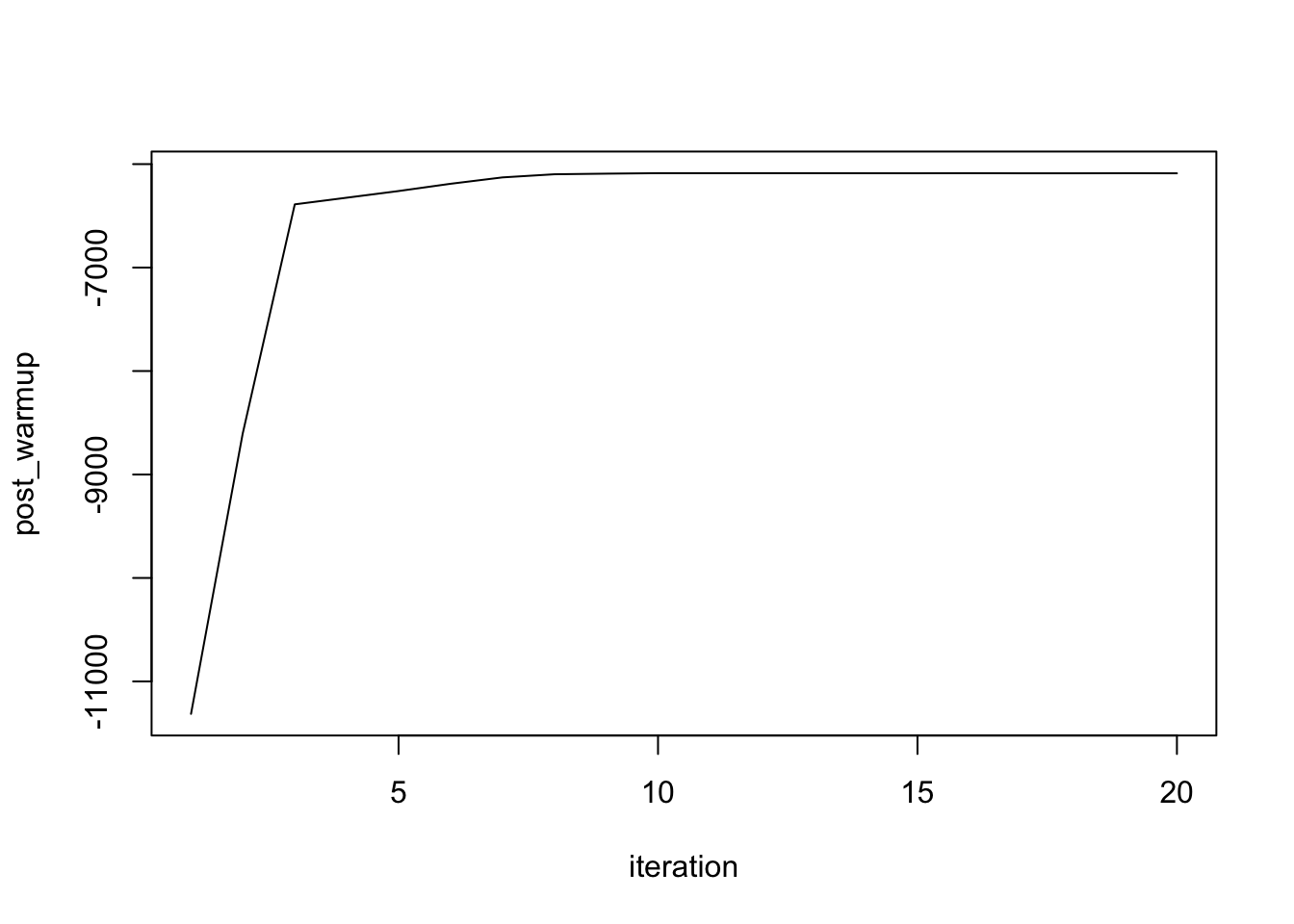
Figure 3.2: check the convergence in warmup period
So HMC has converged based on the current chain. Now, we can set a lower \(L\) to make computation more efficient and decrease the acceptance rate.
L <- 150
epsilon <- signif(1/L,4)

set.seed(2020)
for (i in 21:nrow(chain_HMC)) {
  chain_HMC[i, ] <- HMC(U, grad_U, epsilon, L, chain_HMC[i-1,])
}
Increase L to improve computational efficiency. Another goal is to obtain the optimal acceptance rate in HMC (\(65\%\)).
- Accpetance Rate:
# transform back the constrain parameters
chain_HMC <- t(apply(chain_HMC,1,mcmc_trans_back))

acceptance_HMC <- 1-mean(duplicated(chain_HMC[-(1:50),]))
acceptance_HMC
## [1] 0.78Acceptance Rate between \(60\%\) and \(90\%\) is acceptable in HMC.
- Plot the log-posterior value to see when it converges.
HMC_post <- apply(chain_HMC[1:20,],1,bvn_logposterior)
plot(1:20,HMC_post,type = "l", xlab = "Iteration in HMC",ylab = "log-posterior")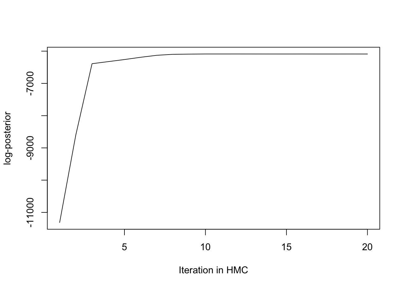
Figure 3.3: Plot the log-posterior value to see when the HMC converges
Figure 3.3 concludes that HMC converges in the first 20 steps, while Figure 3.4 confesses that the Metropolis-Hasting convergence requires around 400 steps to converge. In a nutshell, HMC converges more quickly than MH.
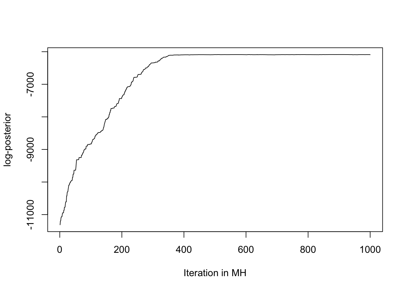
Figure 3.4: Plot the log-posterior value to see when the MH converges
- Compute the Bayesian Estimation for parameters:
# remove burnin steps
chain_HMC <- chain_HMC[-(1:50),]
# compute the Bayesian estimation with 3 digitals
BE_HMC <- round(colMeans(chain_HMC),3)
BE_HMC
## [1] 6.428 1.835 1.420 0.397 0.788- \(95\%\) Credible Inteval:
CI.HMC <- round(apply(chain_HMC, 2, function(x){quantile(x,c(0.025, 0.975))}),3)
colnames(CI.HMC) <- names(parvec)
CI <- rbind(parvec,CI.HMC)
CI
## mu_1 sd_1 mu_2 sd_2 rho
## parvec 6.480 1.850 1.430 0.400 0.800
## 2.5% 6.357 1.794 1.407 0.388 0.775
## 97.5% 6.504 1.878 1.435 0.407 0.802- Histograms and trace plot:
par(mfrow = c(2,3))
hist(chain_HMC[,1],nclass=30, , main=expression(paste("Posterior of ", mu[1])),
     xlab="Bayesian Estimation = red line" )
abline(v = mean(chain_HMC[,1]),col="red" )
hist(chain_HMC[,2],nclass=30, main=expression(paste("Posterior of ", sigma[1])),
     xlab="Bayesian Estimatio = red line")
abline(v = mean(chain_HMC[,2]),col="red" )
hist(chain_HMC[,3],nclass=30, main=expression(paste("Posterior of ", mu[2])),
     xlab="Bayesian Estimatio = red line")
abline(v = mean(chain_HMC[,3]) ,col="red" )
hist(chain_HMC[,4],nclass=30, main=expression(paste("Posterior of ", sigma[2])),
     xlab="Bayesian Estimatio = red line")
abline(v = mean(chain_HMC[,4]),col="red"  )
hist(chain_HMC[,5],nclass=30, main=expression(paste("Posterior of ", rho)),
     xlab="Bayesian Estimatio = red line")
abline(v = mean(chain_HMC[,5]) ,col="red" )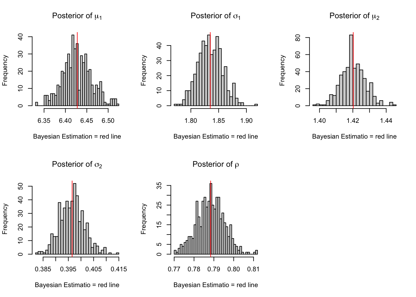
Figure 3.5: Histograms for HMC
par(mfrow = c(2,3))
plot(chain_HMC[,1], type = "l", xlab="Bayesian Estimatio = red line" ,
     main = expression(paste("Chain values of ", mu[1])),ylab = expression(mu[1]) )
abline(h = mean(chain_HMC[,1]), col="red" )
plot(chain_HMC[,2], type = "l", xlab="Bayesian Estimatio = red line" ,
     main = expression(paste("Chain values of ", sigma[1])),ylab = expression(sigma[1]) )
abline(h =  mean(chain_HMC[,2]), col="red" )
plot(chain_HMC[,3], type = "l", xlab="Bayesian Estimatio = red line" ,
     main = expression(paste("Chain values of ", mu[2])), ylab = expression(mu[2]))
abline(h =  mean(chain_HMC[,3]), col="red" )
plot(chain_HMC[,4], type = "l", xlab="Bayesian Estimatio = red line" ,
     main =expression(paste("Chain values of ", sigma[2])), ylab = expression(sigma[2]))
abline(h =  mean(chain_HMC[,4]), col="red" )
plot(chain_HMC[,5], type = "l", xlab="Bayesian Estimatio = red line" ,
     main = expression(paste("Chain values of ", rho)), ylab = expression(rho))
abline(h =  mean(chain_HMC[,5]), col="red" )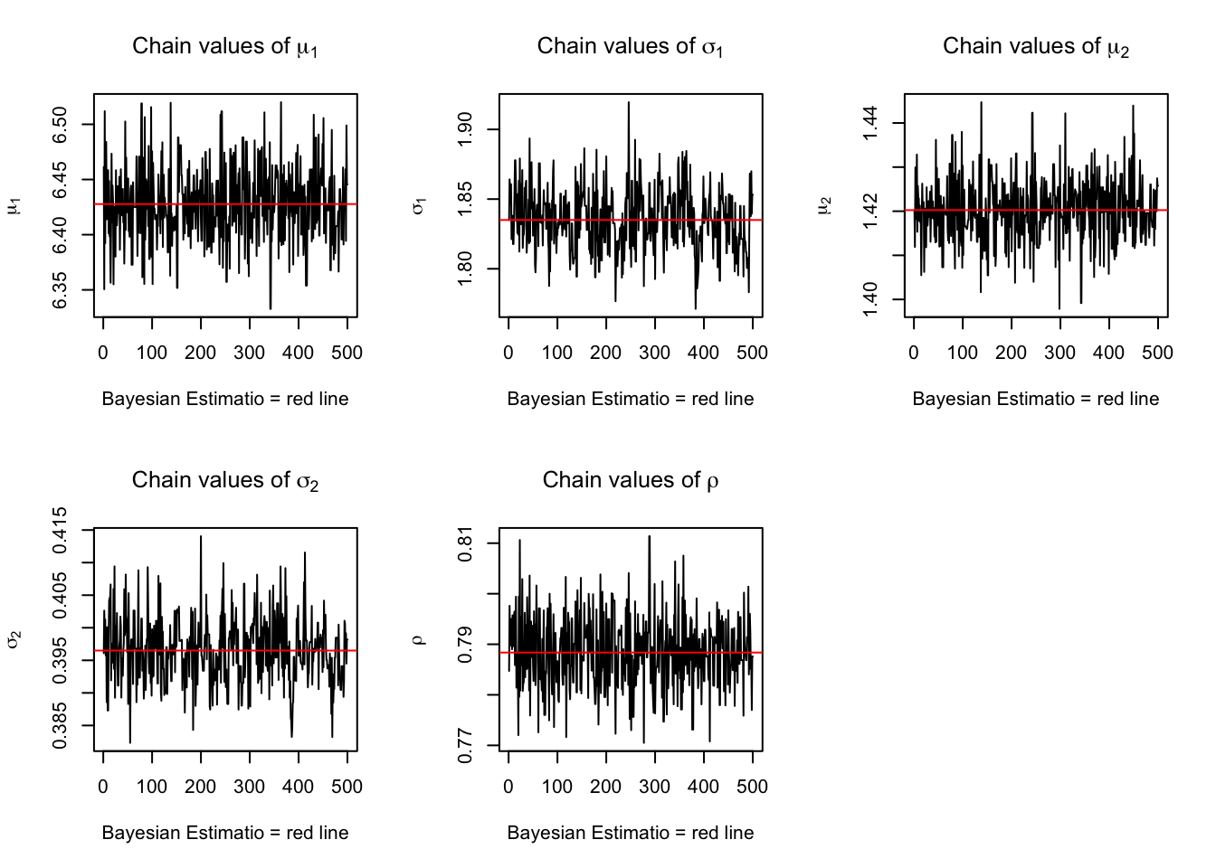
Figure 3.6: trace plots for HMC
library(optimCheck)
theta.names <- c(paste0("mu[1]"),paste0("sigma[1]"), paste0("mu[2]"),
                 paste0("sigma[2]"), paste0("rho")) # pretty names on plot
theta.names <- parse(text = theta.names)
optim_proj(fun = posterior, # objective function
           xsol = BE_HMC, # candidate optimum
           maximize = TRUE,
           xnames = theta.names)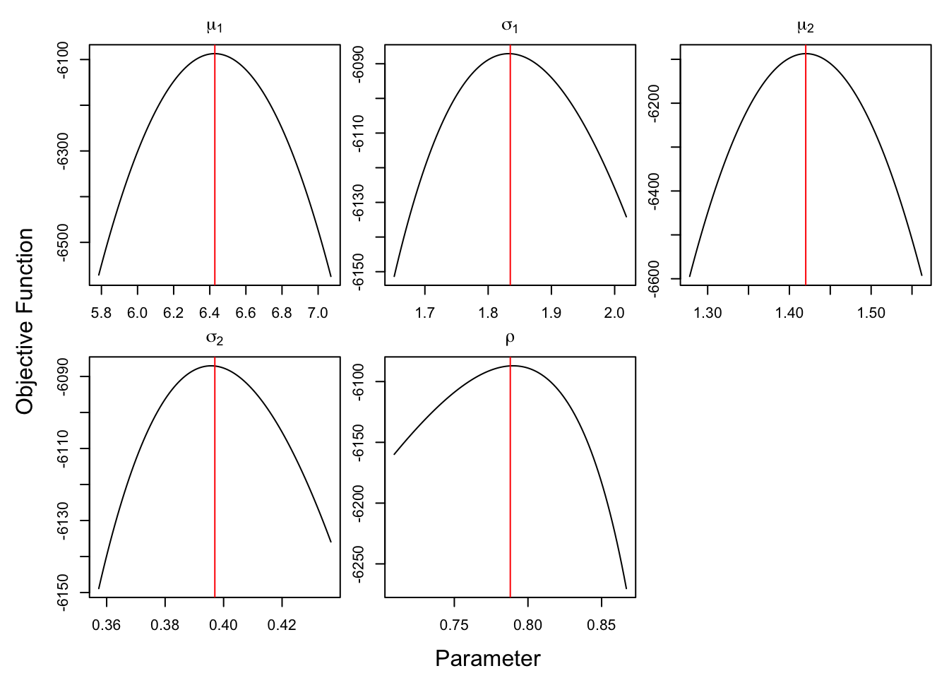
Figure 3.7: check optimization for HMC
Figure 3.7 affirms that all the estimated parameter maximizes the objective functions, i.e. maximizes the posteriors.
HMC can maximize the posterior function.
3.7.4 No-U-Turn Sampler
NUTS (No-U-Turn Sampler) is implemented in Stan. Not only does Stan produce hyper-optimized autodifferentiate C++ code, but it also employs a very effective adaptive tuning mechanism for \(L\). In addition, there is no parameter in NUTS you need to tune. There are many useful tutorial guides in Stan website.
3.7.4.1 Stan Model with Built-in Distribution
Since Stan has defined the multivariate normal disrtibution, we can directly use it in Stan. One of the advantages here is that you will not be bothered by constrained parameters and can directly declare “real<lower=0, upper=1> rho;”.
// The input data is a matrix 'X' of rows 'N'.
data {
  int<lower=0> N;
  matrix[N,2] X;
}

// The parameters accepted by the model.
parameters {
  vector[2] mu;
  real<lower=0> sigma[2];
  real<lower=0, upper=1> rho;
}

transformed parameters{
  matrix[2,2] S; // compute Sigma Matrix
  S[1,1] = sigma[1]^2;
  S[2,2] = sigma[2]^2;
  S[1,2] = sigma[1]*sigma[2]*rho;
  S[2,1] = sigma[1]*sigma[2]*rho;
}

model {
 // prior
  mu[1] ~ normal(6.48,1);
  mu[2] ~ normal(1.43,1);
  sigma[1] ~ normal(1.85,1);
  sigma[2] ~ normal(0.4,1);
  rho ~ uniform(0,1);

  for(i in 1:N){
  X[i,] ~ multi_normal(mu,S);
  }
}
This Stan file is saved as “Bivariate.Stan”.
3.7.4.2 Stan Model with User-defined Function
User-defined function is also provided in Stan, which is more chanllenging than built-in distributions.
Probability functions are distinguished in Stan by names ending in _lpdf for density functions. As with the built-in functions, the suffix _lpdf is dropped and the first argument moves to the left of the sampling symbol (~) in the sampling statement.
Note that Stan is not as “smart” as R in terms of data type. If you do not want matrix computation, it is better to declare your dataset or other variables as real[]. That is why I declare real X[N,2] rather than matrix X[N,2] for my dataset. However, if you want matrix computation, you need to switch it to “vector”. That is why there is “x_vec = to_vector(x)” in the likelihood function. Because inverse_spd() function requires “vector” or matrix as arguments.
// define Bivariate normal distribution
functions {
  // the _lpdf syntax has a special meaning (see below)
  // here x is a 2-d vector so declare it as real[] x;
  // if your x is 1-d number, just declare it as real x.
  real Bi_lpdf(real[] x,vector mu, matrix S) {
    real log_lik; // declare log-likelihood value
    matrix[2,2] inv_s; // declare inverse matrix of S
    real xsx;  // declare quadratic form in the bivariate normal distribution
    vector[2] x_vec; // convert the data into vector

    // convert the data into vector, inverse_spd() require vector or matrix as arguments
    x_vec = to_vector(x);
    // inverse_spd() provide The inverse of A where A is symmetric, positive definite.
    inv_s = inverse_spd(S);
    // quad_from provides The quadratic form, i.e., B'* A * B.
    xsx = quad_form(inv_s, x_vec - mu);

    log_lik = -(log_determinant(S) + xsx);
    return log_lik;
  }
}

data {
  int<lower=0> N;
  real X[N,2];
}

// The parameters accepted by the model.
parameters {
  vector[2] mu;
  real<lower=0> sigma[2];
  real<lower=0, upper=1> rho;
}

transformed parameters{
  matrix[2,2] S; // declare Sigma matrix in the multivariate normal distribution
  S[1,1] = sigma[1]^2;
  S[2,2] = sigma[2]^2;
  S[1,2] = sigma[1]*sigma[2]*rho;
  S[2,1] = sigma[1]*sigma[2]*rho;
}

// The model to be estimated.
model {
  //prior
  mu[1] ~ normal(6.48,1);
  mu[2] ~ normal(1.43,1);
  sigma[1] ~ normal(1.85,1);
  sigma[2] ~ normal(0.4,1);
  rho ~ uniform(0,1);

  for(i in 1:N){
  X[i,] ~ Bi(mu,S);
  }
}
3.7.4.3 Implementation and Analysis of Stan Model
# stan installation instructions:
# https://github.com/stan-dev/rstan/wiki/RStan-Getting-Started
# follow these **EXACTLY** or welcome to error country!

require(rstan)
bi_mod <- stan_model(file = "Bivariate.stan") # compile code
# sampling
# iteration = 2000
bi_fit <- sampling(object = bi_mod,
data = list(N=N,X = bvn),
iter = 2e3)Accessment:
- Posterior draws:
extract() function can return the list of parameters draws from the posterior distribution.
bi_post <- extract(bi_fit)

# show some draws of mu
head(extract(bi_fit)$mu)
##
## iterations [,1] [,2]
## [1,] 6.422246 1.424042
## [2,] 6.338986 1.413239
## [3,] 6.406891 1.410834
## [4,] 6.409214 1.413599
## [5,] 6.430308 1.420195
## [6,] 6.460905 1.420322- Convergence and posterior statistics:
theta <- c("mu","sigma", "rho") #Define the theta
print(bi_fit, pars = theta)
## Inference for Stan model: Bivariate.
## 4 chains, each with iter=2000; warmup=1000; thin=1;
## post-warmup draws per chain=1000, total post-warmup draws=4000.
##
## mean se_mean sd 2.5% 25% 50% 75% 97.5% n_eff Rhat
## mu[1] 6.43 0 0.03 6.36 6.41 6.43 6.45 6.49 2250 1
## mu[2] 1.42 0 0.01 1.41 1.42 1.42 1.42 1.43 2425 1
## sigma[1] 1.83 0 0.02 1.79 1.81 1.83 1.85 1.88 2481 1
## sigma[2] 0.40 0 0.01 0.39 0.39 0.40 0.40 0.41 2621 1
## rho 0.79 0 0.01 0.77 0.78 0.79 0.79 0.80 2760 1
##
## Samples were drawn using NUTS(diag_e) at Fri Jun 5 11:59:11 2020.
## For each parameter, n_eff is a crude measure of effective sample size,
## and Rhat is the potential scale reduction factor on split chains (at
## convergence, Rhat=1).All the Rhat = 1 shows the NUTS converges. The summary includes the posterior mean, the posterior standard deviation, and various quantiles computed from the draws.
Moreover, the effective sample size (ESS) is a more quantitative measure, which approximates the number of iid samples to which the correlated MCMC samples correspond. As a general rule-of-thumb each ESS should be at least 400.
- Trace plot:
stan_trace(bi_fit, pars = theta, xnames = theta.names) # Trace plot per parameter## Warning in ggplot2::geom_path(...): Ignoring unknown parameters: `xnames`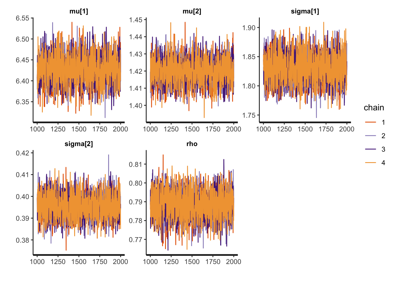
Figure 3.8: trace plots for NUTS
The chains completely overlap with each other, which is evidence that the MCMC has converged. However, we have got the list of parameter draws in (1). We can use similar ways in MH and HMC to obtain trace plots and histograms.
- Parameters Density:
stan_dens(bi_fit, pars = theta, separate_chains = TRUE)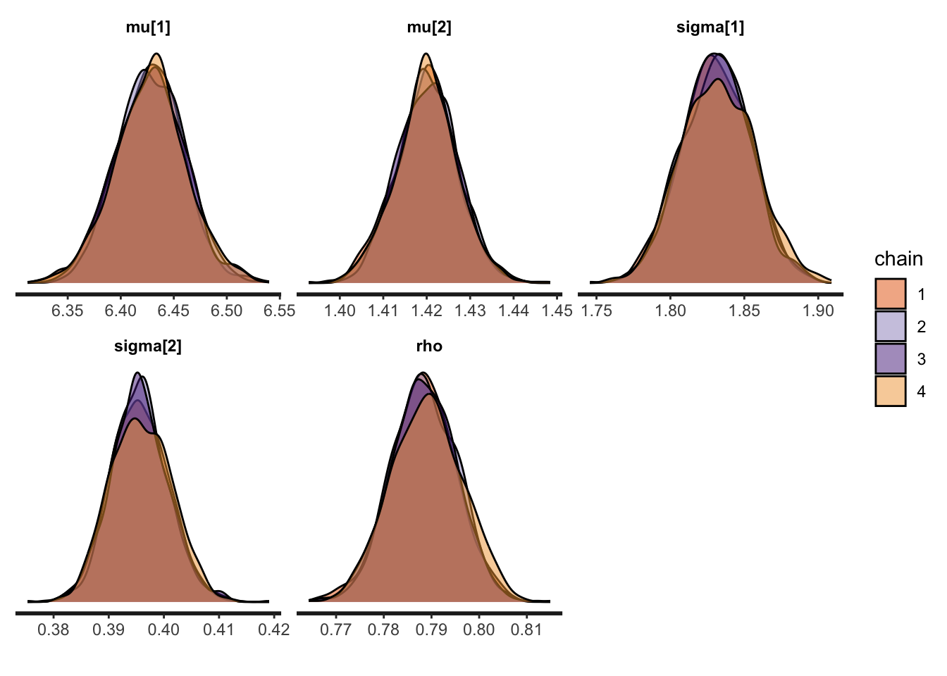
Figure 3.9: Density plots for NUTS
rstan::stan_dens() provides the density per parameter for each chain which is very helpful for diagnosis.
- histograms:
pairs(bi_fit, pars = theta, cex.labels = 1)## Warning in par(usr): argument 1 does not name a graphical parameter
## Warning in par(usr): argument 1 does not name a graphical parameter
## Warning in par(usr): argument 1 does not name a graphical parameter
## Warning in par(usr): argument 1 does not name a graphical parameter
## Warning in par(usr): argument 1 does not name a graphical parameter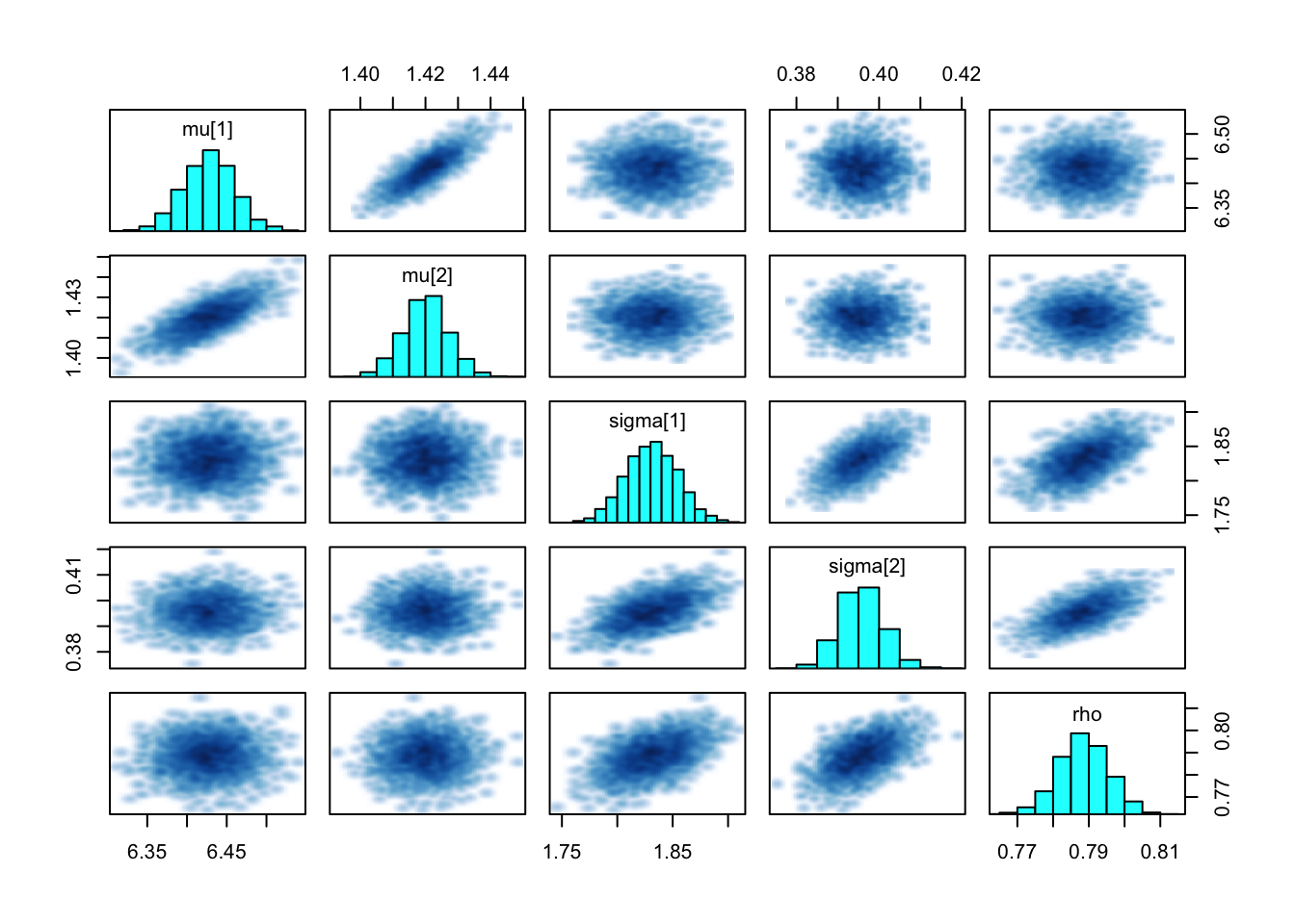
Figure 3.10: Histograms for NUTS
rstan::pairs() provides the histograms and scatterplots for analysis. Here, all the parameters show univariate normal distribution, which is corresponding to theory.
3.8 Stan examples
To facilitate understanding how to use Stan, two examples4 will be provided in this section to give a step-by-step guide.
Useful resources online are listed below:
Stan Installation provides a quick tutorial for downloading, installing, and getting started with RStan on all platforms.
Stan user guide is the official user’s guide for Stan and provides examples for coding statistical models in Stan.
Stan function reference provides a list of defined functions and distributions in the Stan math library and available in the Stan programming language.
3.8.1 Sigma Mean-Variance Normal
The inference of for the sigma mean-variance Normal model is given by \(\sigma \sim p(\sigma\mid y)\), where
\[ \sigma \sim \chi^{2}_{(7)}, \quad y_{i}\mid \sigma \iid \N(\sigma,\sigma^{2}) \]
3.8.1.1 Step 1: Complie the Stan Model
The distributions involved in this model are available in the Stan library and can be called directly in “model” block. The Stan code for this model is given as follows.
data {
  int<lower=0> N; // sample size
  real y[N]; // y1, ..., yN
}
parameters {
  real<lower=0.00001> sigma; // sigma restricted to be positive
}
model {
  sigma ~ chi_square(7); // prior
  y ~ normal(sigma, sigma); // likelihood
}
In the “data” block, we declare real y[N] rather than vector y[N] since no linear algebra computation is engaged. You can paste the following code as a Stan file named “SigmaMeanVarModel.stan” and compile the model with the following code.
require(rstan) # load the package
# Compile the stan model
sigmv_mod <- stan_model(file = "SigmaMeanVarModel.stan")
Note that lots of warnings may come up in this step, but most of them can be ignored.
3.8.1.2 Step 2: Construct the Log-posterior
As preparatory work for next step, the following code simulates data and constructs the log-posterior of the data in Stan.
Two steps to instantiate the model corresponding in the Stan files with some simulated data are:
Format the data: list the data with elements exactly ad the “data” block in Stan file.
Associate the data with model with one iteration MCMC sample.
# Simulate data
sigma <- rexp(1) + 5
N <- 1e2
y <- rnorm(N, sigma, sigma)

# Construct log-posterior for this data in Stan
# 1. format data:
#   list with elements named exactly as "data" block in Stan
sigmv_data <- list(N = N, y = y)

# 2. associate data with model:
# to do this, MCMC sample for one iteration.
# here I initialized the sampler from a reasonable value, to avoid
# errors due bad random starting points.
sigmv_fit <- sampling(sigmv_mod, data = sigmv_data, iter = 1,
                      verbose = TRUE, chains = 1,
                      init = list(list(sigma = 10)))
3.8.1.3 Step 3: Correctness of Stan
To ensure integrity, the Stan code shall be tested in the first place. For generic MCMC, checking that log-posterior is correct will suffice, which can be realized with log_prob and expose_stan_functions functions in rstan package.
The model parameters are firstly generated arbitrarily. It’s expected that the R log-posterior and Stan log-posterior at these values differ by a constant. This constant is the summation of the constant additive term of the posterior, as these terms will be dropped by default in Stan.
# simulate some parameter values:
# here's a Stan compatible approach for doing this
nsim <- 18 #number of simulation
Pars <- replicate(n = nsim, expr = {
  list(sigma = 3*rexp(1))
}, simplify = FALSE)

# Unnormalized log-posterior distribution in R:
# since you're testing against this, write it as transparently as possible
# to minimize the chance of error.
# Pay zero regard to speed considerations.
logpost <- function(sigma, y) {
  lp <- dchisq(sigma, df = 7, log = TRUE) # prior
  lp + sum(dnorm(y, mean = sigma, sd = sigma, log = TRUE)) # likelihood
}

# log-posterior in R:
lpR <- sapply(1:nsim, function(ii) {
  sigma <- Pars[[ii]]$sigma
  logpost(sigma, y = sigmv_data$y)
})

# log-posterior in Stan:

# Note that Stan samples on an "unconstrained scale", i.e., transforms
# all positive parameters to their logs and samples on that scale.
# however, results are typically returned on the regular scale.
# to fix this use the adjust_transform argument.

# ?log_prob for details, though at present
# adjust_transform is incorrectly documented
# (definition for TRUE and FALSE reversed)
# (and that's why you should ALWAYS check other ppl's code)
lpStan <- sapply(1:nsim, function(ii) {
  upars <- unconstrain_pars(object = sigmv_fit, pars = Pars[[ii]])
  log_prob(object = sigmv_fit, upars = upars, adjust_transform = FALSE)
})


lpR-lpStan # should return a vector of identical values.
-log(gamma(7/2)*2^(7/2))-log(sqrt(2*pi))*N # additive terms of posterior
3.8.1.4 Step 4: Compare MCMC to True Posterior
The attraction of simulation study is that the true posterior is available such that we can evaluate the performance of the MCMC.
# On my computer it takes several tries before the 1st draw is accepted
# without throwing an error, but if 1st draw is accepted for some reason
# after that all nsamples draws work fine.
nsamples <- 1e5
sigmv_fit <- sampling(sigmv_mod, data = sigmv_data, iter = nsamples,
                     chains = 1,
                     init = list(list(sigma = 10)))
# extract MCMC samples
sigmv_post <- extract(sigmv_fit)
names(sigmv_post) # lp__ is the log-posterior at each iteration
sigma_post <- sigmv_post$sigma # MCMC output

# Histogram of MCMC samples
hist(sigma_post, breaks = 100, freq = FALSE,
     xlab = expression(sigma), main = expression(p(sigma*" | "*bold(y))))
# Add analytic output to the histogram
sigma_seq <- seq(min(sigma_post), max(sigma_post), len = 200)
sigma_pdf <- sapply(sigma_seq, logpost, y = sigmv_data$y) # logposterior
sigma_pdf <- exp(sigma_pdf - max(sigma_pdf)) # normalize
# I typically do this in two steps to minimize roundoff errors
sigma_pdf <- sigma_pdf/sum(sigma_pdf)/(sigma_seq[2]-sigma_seq[1])
lines(sigma_seq, sigma_pdf, col = "red")
legend("topright", col = "red", "True Posterior", lty = 1)# add legends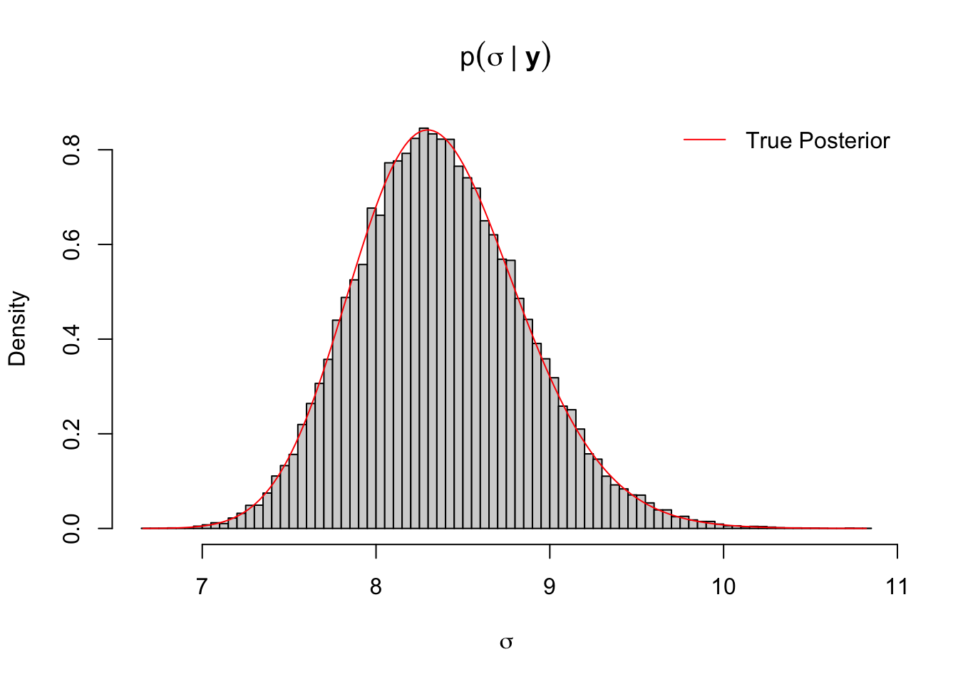
Figure 3.11: Histogram of MCMC output of sigma mean-variance normal model with true posterior density curve
It can be concluded from Figure 3.11 that the histogram of MCMC samples fits the true posterior well and the MCMC output converges.
3.8.2 Banana distribution
The previous example utilizes the built-in functions in Stan library. When such functions are unavailable in the Stan library, the posterior shall be defined manually in Stan file.
The posterior of the banana distribution model for each observation \((x_{1},x_{2})\)is defined as: \[ p(x_{1},x_{2}|y,\sigma) \propto \exp\{-\frac{1}{2}[\frac{(y-x_{1}x_{2})^{2}}{\sigma} + (x_{1} - x_{2} )^{2}]\}. \]
3.8.2.1 Step 1: Complie the Stan Model
In the Stan file, the log-posterior is firstly defined in “functions” block.
// sampling from the Banana distribution
// here is your log-likelihood distribution
functions {
  // banana distribution (unnormalized)
  // the _lpdf syntax has a special meaning (see below)
  real Banana_lpdf(real[] x, real y, real tau) {
    real yx;
    real xx;
    yx = y-x[1]*x[2];
    xx = x[1]-x[2];
    return -.5 * (yx*yx*tau + xx*xx);
  }
}

data {
  real<lower=0> sigma;
  real<lower=0> y;
}

transformed data {
  real<lower=0> tau;
  tau = 1.0/(sigma*sigma);
}

parameters {
  real<lower=0> x[2];
}

model {
  // these two statements have identical effect
  // target += Banana_lpdf(x, y, tau); // access "target" distr. directly
  x ~ Banana(y, tau); // prefered stan method (see reference manual)
}
This file can be saved as “BananaDistribution.stan” such that the follow code will compile the model.
ban_mod <- stan_model(file = "BananaDistribution.stan") # compile code3.8.2.2 Step 2: Correctness of Stan
First of all, the log-posterior of this example needs to be explicitly defined in R as well.
# unnormalized log density in R
lbanana <- function(x) {
  -.5 * ((y-x[1]*x[2])^2/sigma^2 + (x[1]-x[2])^2)
}
The Stan file contains a custom function (defined in “functions” block) called Banana_lpdf corresponding to the Banana log-distribution. The following code is to test this custom Stan functions. Here we expect the difference to be small numbers around 0.
# banana parameters
sigma <- .1
y <- .3
# Exports all custom functions to R workspace:
expose_stan_functions(stanmodel = ban_mod)
Banana_lpdf # the only exported function in this case is Banana_lpdf

# check output
npts <- 200
xseq <- seq(0, 3, len = npts)
X <- as.matrix(expand.grid(xseq, xseq))
Xtest <- X[sample(nrow(X), 20),] # random points from 2d grid

# log-posterior in R
ldR <- apply(Xtest, 1, lbanana)

# log-posterior in Stan
ldStan <- apply(Xtest, 1, function(x) {
  Banana_lpdf(x, y = y, tau = 1/sigma^2)
})

ldR - ldStan # check difference
3.8.2.3 Step 3: Compare MCMC to True Posterior
Similar to the previous example, the MCMC sampling can be implemented with the following code.
# MCMC sampling
ban_fit <- sampling(object = ban_mod,
                    data = list(y = y, sigma = sigma),
                    iter = 1e4)
ban_post <- extract(ban_fit) # extract the output
To visualize the results, the histogram of MCMC samples and the analytic posterior can be plotted by the following code.
# superimpose contours on scatterplot and 1-d posterior on histogram
par(mfrow = c(1,2), mar = c(4,4,2,.5)+.1)
Xpdf <- matrix(apply(X, 1, lbanana), npts, npts)
Xpdf <- exp(Xpdf-max(Xpdf))
xpdf <- rowSums(Xpdf) # summing over x2, i.e., get f(x1)
xpdf <- xpdf/sum(xpdf)/(xseq[2]-xseq[1]) # normalize
# 2-d contour
plot(ban_post$x[1:2e3,], pch = 16, cex = .5,
     xlab = expression(x[1]), ylab = expression(x[2]),
     main = expression(p(x[1],x[2])))
contour(x = xseq, y = xseq, z = Xpdf,
        add = TRUE, col = "red", lwd = 2, nlevels = 5)
# 1-d marginal (same for both variables)
hist(ban_post$x[,1], breaks = 100, freq = FALSE,
     xlab = expression(x[1]),
     main = expression(p(x[1])))
lines(xseq, xpdf, col = "red", lwd = 2)
legend("right", col = "red", "True Posterior", lty = 1, cex = 1, bty='n')# add legends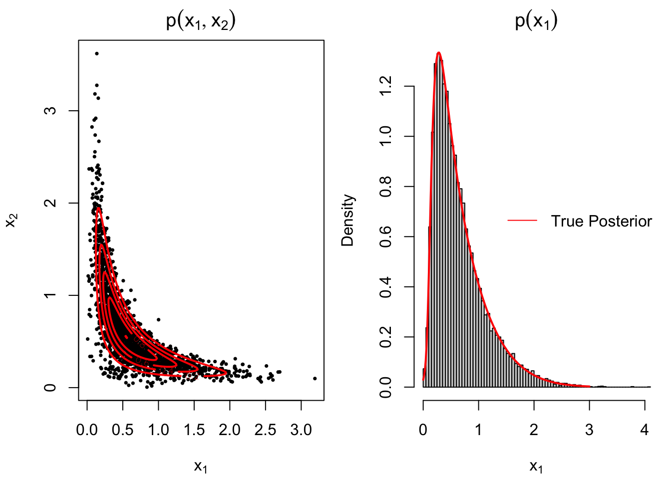
Figure 3.12: 2-dimensional contour plot and 1-dimensional marginal of MCMC output of Banana distribution with true posterior density curve
Note that the marginal density for both variables are the same and only the output for \(x_1\) will be displayed for inference. It can be concluded from Figure 3.12 that the histogram of MCMC samples fits the true posterior well and the MCMC output converges.