Chapter 9 Approximate Bayesian Computation
9.1 Introduction
Approximate Bayesian Computation, or ABC for short, is a family of computational methods/algorithms that is used to approximate the probability distributions of a function given its estimated posterior distribution. Often in time the likelihood function is derived for the calculation but in many more complicated real world scenarios such as spread of bacteria (Fearnhead and Prangle 2012) the exact likelihood function might be nearly impossible to obtain due to the limited amount of computation power available, and this is where the ABC algorithms comes in.
ABC methods bypass the usage of likelihood function thus is less expensive to use but at the same time result obtained will not be as precise.
ABC is becoming a more popular tool for analysis due to the increase of data’s complexity in recent years. The ABC algorithms are greatly involved in areas such as genetics, biology, and epidemiology(M. G. B. Blum et al. 2012).
9.2 General Idea
The goal for ABC algorithms is to draw samples without using the likelihood function, which can translate into finding \(P(\theta|X = X_{observed})\) where X is the dataset, and \(\theta\) is the corresponding model parameters.
The training data we need to generate can be denoted as \((X_1,\theta_1),(X_2,\theta_2)...(X_m,\theta_m)\) where \(P(X,\theta) = P(X|\theta)*\Pi(\theta)\) where \(\Pi(\theta)\) is the prior according to conditional probability.
When we reserves engineering and work backward, we can also write \(P(X,\theta) = P(\theta|X)^P(X)\). This is saying that term \(P(X,\theta)\) is the product of the “evidence” and the posterior.
Going back to our training data we can have the following \(X_i ~ iid P(X)\) and \(\theta_i|X_i ~ ind P(\theta|X_i)\). This means that the \(\theta_i\) term is just the posterior distribution given \(X_i\) pairs! We’ve found a way to bypass the likelihood function to solve for posterior distribution!
9.3 ABC Main Algorithm
Due to the rise in popularity for ABC algorithms in recent years researchers have developed many modified version of ABC procedures that are offer slight increase in accuracy and/or decrease in the computation duration. None the less all variations are based on the original idea first proposed by Diggle & Gratton in 1984 where they first proposed a method to set simulation to do statistical inference where the likelihood function is intractable. Although the idea was proposed back then it has not gotten too much attention until recent years due to the lack of computation power back then.
The Main ABC algorithm can be divided into 4 steps: Generate training data, rejection of training data, regression adjustment and sampling from posterior. Each steps will be briefly talked about and pseudo-code written in R Studio will be used to showcase all the intermediate steps to enhance reader’s understanding.
9.3.1 Step 1: Generating Training Data
The first step of any ABC algorithms is to generate sample training data, where \(X_{ii}\) is \(ii^ {th}\) the outcome term of the training data, \(\theta_{ii}\) is the \(X_{ii}\)’s corresponding parameters and the term n_train_full indicates how many samples are being generated. Pseudo-code for part one is shown below:
# Step 1: generate training data
n_train_full <- 1e5

# preallocate memory
theta <- matrix(NA, n_train_full, n_theta)
X <- matrix(NA, n_train_full, n_X)

for(ii in 1:n_train_full) {
  theta[ii,] <- prior_sim() # theta_i ~iid pi(theta)
  X[ii,] <- data_sim(theta = theta[ii,]) # X_i | theta_i ~ind p(X | theta_i)
}
9.3.2 Step 2: Implementing Rejection Algorithm
In part 1 we generated a number of samples, however not all the samples generated from part 1 are similar to the observed data. If we keep all the sample data generated from part 1 and proceed we will not receive an accurate estimate. Therefore, the rejection algorithm must be implemented to compare each sample and make sure they are similar to the observed value. Term \(\epsilon\) is used as the threshold value to either accept or reject a particular sample value. \(\epsilon\) can be interrupted as the Euclidean distance (or other distance measurement of user’s own choice) between the sampled data and the observed data. Small \(\epsilon\) value implies that the training data can be accepted only if it is very alike the observed data, thus using small \(\epsilon\) value will give us a more precise result but at the same time since more points are being rejected, the algorithm will take much longer to accept enough points. On the other hand, if we set \(\epsilon\) value to be very large then the rejection algorithm will still accept samples that are not as quite as the same as the observed data. In return we will likely see a less accurate result but a much faster run-time. Generally speaking, a low dimensional and near sufficient s would provide a near optimal and balanced choice between the two.
To simplify the \(\epsilon\) value selection, one can instead pick the percentage of training sampled to accept. In this example we generated \(10^5\) samples in part one and instead of coming up with a magical \(\epsilon\) value we decided to keep \(10^4\) samples (accept 10 percent) and reject the rest, sorted by their individual \(\epsilon\) values.
# Step 2: rejection
# often it's easier to specify fraction of samples you keep
# rather than epsilon directly
n_train <- 1e4 # how many samples to keep after rejection
S <- matrix(NA, n_train_full, n_S)
for(ii ni 1:n_train_full) {
  S[ii,] <- summary_stat(X[ii,])
}

# summary statistics for observed data
S_obs <- summary_stat(X_obs)

# whatever distance you want, probably euclidian
S_dist <- dist(S, S_obs)

# returns indices on n_train smallest values
keep_id <- which_min(S_dist, n = n_train)
X <- X[keep_id,]
theta <- theta[keep_id,]
9.3.3 Step 3: Applying Regression Adjustment
Step 3 is to take the accepted sample pairs from part 2 and perform regression adjustment for generalization. The concern we have with the sampling part alone is that we can have the most optimal initial setup but the chances of us getting the exact same sample points as the observed points are nearly zero. Regression adjustment is used to adjust parameters of \(\theta_{ii}\) with non-zero weight \(w_{ii}\) in order to account the imperfection between the generated value and the observed value and make our training sample more flexible (M. G. Blum 2017). The simplest linear regression model can be represented as \(y_{m} = x^{'}_m\beta_{p*d}+\epsilon_{m}\). Before this step it is highly recommended to perform normalization of the accepted samples. Reason for this is that after the rejection algorithm the probability density function will no longer add up to 1 and the distribution may not be a normal distribution. The purpose of the normalization is to recover the sum of its pdf back to 1.
# Step 3: regression adjustment
# to do this properly, it's much easier if we pre-transform the data to be marginally N(0,1).
#' Transform input to quantiles of the standard normal.
#' @param x Vector of values to transform.
#' @param xdata Vector of values from which to compute the empirical CDF.
#' @return Map of the rank of each `x` in `xdata` to the corresponding quantile of a `N(0,1)`.
norm_trans <- function(x, xdata = x) {
  rnk <- sapply(x, function(xi) sum(xi <= xdata))/(length(xdata)+1)
  qnorm(rnk)
}

#' Inverse of `norm_trans()`.
#' @param z Vector of normal quantiles.
#' @template param-xdata
#' @return Maps each `z` to the corresponding quantile of `xdata`.
norm_itrans <- function(z, xdata) {
  quantile(xdata, prob = pnorm(z), names = FALSE)
}

# step 3a: "normalize" everything.
# apply norm_trans to each column of X and theta
X_z <- apply(X, 2, norm_trans)
theta_z <- apply(theta, 2, norm_trans)

# step 3b: regression
beta_hat <- matrix(NA, n_X, n_theta)
eps <- matrix(NA, n_train, n_theta)
for(ii in 1:n_theta) {
  M <- lm(theta_z[,ii] ~ X_z - 1) # remove intercept since everything is centered at 0
  beta_hat[,ii] <- coef(M)
  eps[,ii] <- resid(M) # theta_z[,ii] - lm_prediction
}
9.3.4 Step 4: Sampling from Posterior
Everything is all set up. we can then sample outcomes using information obtained above and despite the intractable likelihood function!
# step 4: sample from the posterior
# step 4a: sample with replacement from the rows of eps.
n_samples <- 1e5
post_id <- sample(n_train, size = n_samples, replace = TRUE)
eps_post <- eps[post_id,]
# step 4b: add the regression mean to each eps.
# transform each element of X_obs the same as we did for each column of X
X_obs_z <- sapply(1:n_X, function(ii) {
  norm_trans(x = X_obs[ii], xdata = X[,ii])
})

mu_hat <- X_obs_z %*% beta_hat # 1 x n_theta matrix
theta_z_post <- t(t(eps_post) + c(mu_hat)) # add each element of mu_hat to each column of eps_post
# step 4c: transform back to orginial posterior scale
theta_post <- sapply(1:n_theta, function(ii) {
  norm_itrans(x = theta_z_post[,ii], x = theta[,ii])
})
9.4 Problem Description
Copulas are a group of multivariate distribution functions with standard uniform uni-variate margins. The Copula functions are used to describe the dependency between multiple variables. The concept of Copula functions are first proposed by Sklar (Marius and Machler 2011). In recent years Coupula functions has gained attention in fields such as quantitative fiance(Rad, Low, and Faff 2016), reliability engineering (Wu 2014), and signal processing (Qian et al. 2017).
Archimedean Copula is a type of Coupula function that can be further separated by individual families such as Clayton Coupula, Frank Coupula and other Coupula. The concept of Copula is somewhat complicated and since the focus of this chapter is on the explanation of Approximation of Bayesian Computation, details for Copula functions will not be discussed. Readers are encouraged to perform self research on Copula functions in time permits.
It is required to have implement some kind of measurement for the degree of dependency between each individual random variables. Such measurement is known as the measures of association and Kendall’s tau value is often used to represent this association. The Kendall’s tau value is defined as \(\tau = E[sign((X_1 - X_1^{'} )(X_2 - X_2^{'}))]\), where \(\tau = P( (X_1-X_1^{'}) (X_2 - X_2^{'}) >0 ) - P( (X_1-X_1^{'}) (X_2 - X_2^{'}) <0 )\)
Where the value \(\tau\) is a real number ranging from -1 to +1 that measures the probability with which large values of one variable are associated with the large values of other variable. Different type of Copula functions will have different equation to calculate \(\tau\) value. Again since the focus of this chapter is on ABC, detailed explanation of Kendall’s tau will not be discussed.
Figure 9.1 compares five bi-variate copulas for different values of Kendall’s \(\tau\). The .Rmd file also shows how to set figures in R Markdown:
## Loading required package: copula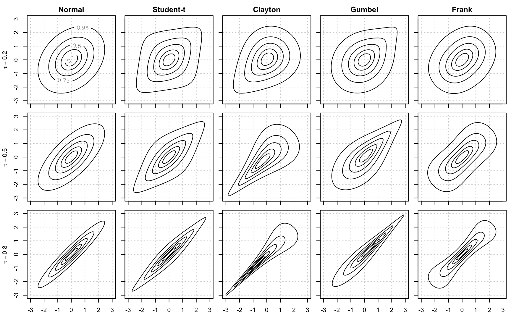
Figure 9.1: Comparison of different copula families for different values of Kendall’s \(\tau\)
A d-dimensional Copula C is called Nested Archimedean Copula if one Archimedean Copula contains complete or partial entry for other Archimedean Copula functions. In other words, the Nest Archimedean Copula functions recursively apply itself to its child Copula function, and this can be demonstrated using a tree diagram. A simple 2-level NAC \(C(\UU_1, \UU_2, \mid \tta)\), where \(\UU_i = (U_{i1}, \ldots, U_{id_i})\) and \(\tta = (\tau_0, \tau_{11}, \tau_{21})\), is represented by the following diagram Figure 9.2:
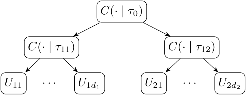
Figure 9.2: Tree representation of a 2 level NAC function
Suppose we have an independent and identically distributed samples from a d-dimensional NAC copula such that \(\cU = (\UU_1, \ldots, \UU_n)\), \(\UU_i = (U_{i1}, \ldots, U_{id})\), where\(\UU_i \iid p(\UU \mid \tta),\) \(\UU_{ij} \sim \unif(0,1)\), and \(\tta = (\tau_1, \ldots, \tau_p)\) are the model’s Kendall-\(\tau\) parameters.
Prior Distribution: Must be able to generate iid samples from \(\pi(\tta)\). A simple choice is constrained uniforms, i.e., for a 2-level NAC with \(\tta = (\tau_{00}, \tau_{11}, \tau_{12})\), such that \(0 < \tau_{00} < \tau_{11}, \tau_{12} < 1\), the constrained uniform prior is \[ \begin{aligned} \tau_{1k} & \iid \unif(0,1) \\ \tau_{00} \mid \tau_{11}, \tau_{12} & \sim \unif\left(0, \min\{\tau_{11}, \tau_{12}\}\right) \end{aligned} \]
Our objective is to obtain the posterior distribution for this 2-level NAC function. According to Bayesian theorem we can obtain the posterior distribution using \(p(\tta \mid \cU_\obs) \propto p(\cU_\obs \mid \tta) \cdot \pi(\tta)\). However this is very difficult to do so because the fact that \(p(\cU \mid \tta) = \prod_{i=1}^n p(\UU_i \mid \tta)\) for NAC models typically cannot be computed efficiently. As one could imagine, NAC functions are complicated in nature and the likelihood function for each tau value is intractable; ABC algorithms can be applied to situation like this to estimate the posterior function for each \(\tau\) value.
In this example we will demonstrate how ABC is implemented onto a 2-level Nested Archimedean Copula to estimate the posterior for each \(\tau\) values.
9.5 Numerical Implementation
9.5.1 Initiation/Environment Setup
Code below are written in nacop-abc-simulate.R
We will work with a 2-level NAC model and attempt to estimate it’s posterior distribution using ABC algorithm defined in previous section. We set the parameter(i.e Kendall’s tau values) alongside with their corresponding prior distributions mentioned above. In terms of the true value we set them to be 0.4, 0.7 and 0.9 respectively. We choose the Clayton 2-level NAC model that includes 250 observations with 5 dimensions and 15 dimensions on each of its block respectively. The code block shown below are used to initiate parameters mentioned above. Please note that all the helper functions will be listed in the appendix section.
#' # Environment Setup
#' You will need a number of packages for this.  If you don't have a particula package installed, then first run e.g., `install.packages("copula")`.
require(copula) # load the package
require(pcaPP) # for sufficient statistics (see below)
require(partitions) # needed internally for "nacop-functions.R"
source("nacop-functions.R") # helper functions

# true parameter values
copfam <- "Clayton" # copula family
tau_true <- c(tau_00 = 0.4, tau_11 = 0.7, tau_12 = 0.9)

# data specification
n_obs <- 250 # number of iid observations
d_11 <- 5 # dimensions of first nested block
d_12 <- 15 # dimensions of second nested block

# generate the observed dataset
U_obs <- sim_nac(n_obs = n_obs, d_11 = d_11, d_12 = d_12,
                 tau_00 = tau_true[1], tau_11 = tau_true[2],
                 tau_12 = tau_true[3], copfam = copfam)
9.5.1.1 Step 1 and 2 Generation of Training Data
Following the ABC procedure listed above, we first have to simulate the training data for our 2-level Clayton NAC model followed right after with a rejection algorithm that only allow us to keep the training data that are similar to our observed value. The accepted samples are then consolidated and saved into an csv file. We set the number of training samples to be \(10^4\) while having a rejection rate of 0.95. As mentioned in the pseudo-code section above, we will specify the percentage of rejection samples instead of declaring the actual \(\epsilon\) to simplify the process. In order to further speed up this process samples will be generated and evaluated in batches.
# simulation parameters
n_train <- 1e4 # number of training samples _after_ rejection
reject_rate <- .95 # fraction of samples to reject per batch
batch_size <- 1e4 # size of each batch
# number of batches needed to get n_train
n_batches <- n_train/(batch_size * (1-reject_rate))
tauhat_obs <- kendall_tau(U_obs) # summary statistics for U_obs

# helper function to simulate one batch and apply rejection sampler
# output is a list of with elements `tau` and `tauhat` consisting of
# matrices with `out_size = batch_size * (1-reject_rate)` rows each.
batch_sim <- function(batch_size, out_size, tauhat_obs) {
  # generate tau from the prior: tau ~ pi(tau)
  tau_batch <- cbind(tau_00 = runif(batch_size),
                     tau_11 = runif(batch_size),
                     tau_12 = runif(batch_size))
  # tau_00 is renormalized to satisfy the constraint
  tau_batch[,1] <- tau_batch[,1] * pmin(tau_batch[,2], tau_batch[,3])
  # generate U from the NAC model: U ~ p_NAC(U | tau)
  U_batch <- lapply(1:batch_size, function(ii) {
    sim_nac(n_obs = n_obs, d_11 = d_11, d_12 = d_12,
            tau_00 = tau_batch[ii,1], tau_11 = tau_batch[ii,2],
            tau_12 = tau_batch[ii,3], copfam = copfam)
  })
  # sometimes the NAC simulation fails.  let's eliminate those samples
  bad_id <- sapply(U_batch, anyNA)
  U_batch <- U_batch[!bad_id]
  tau_batch <- tau_batch[!bad_id,]
  # calculate Kendall's tau for each sample
  tauhat_batch <- lapply(U_batch, kendall_tau)
  # keep the out_size samples closest to tauhat_obs
  tauhat_dist <- sapply(tauhat_batch,
                        function(tauhat) sqrt(sum((tauhat - tauhat_obs)^2)))
  keep_id <- order(tauhat_dist)[1:out_size]
  list(tau = tau_batch[keep_id,],
       tauhat = do.call(rbind, tauhat_batch[keep_id]))
}
A simple for loop is used to loop through the batches to perform rejection algorithm. This is a fairly lengthy process and it may take around 1 minute per batch. In our setup we chose to work with 20 batches thus it will take approximately 20 minutes for code below to execute. We are aware of this long runtime thus had made a saved copy of the value generated. The code block listed below will not be executed to save us time. Readers can execute the following code block by changing the eval=FALSE to TRUE.
Please note that this operation is performed using a single core CPU and can be further optimized with the usage of multi-core CPU. For our demonstration purpose this multi-core is not required; readers are encouraged to research on how multi-core operation is executed in R Studio.
U_train is a matrix with dimension of \(n_{obs} * (d_{11}+D_{12})\) which contains all the observation values for each \(\tau\) outcome. It is then converted into their summary statistics matrix which is denoted as ‘tauhat’. ‘tauhat’ is the summary statistics of the original observations thus its dimension will be smaller than the original one.
# for-loop over batches
tau_train <- vector("list", n_batches) # allocate memory
tauhat_train <- vector("list", n_batches)
for(ii in 1:n_batches) {
  message("Batch ", ii, "/", n_batches)
  tmp <- batch_sim(batch_size = batch_size,
                          out_size = batch_size * (1-reject_rate),
                          tauhat_obs = tauhat_obs)
  tau_train[[ii]] <- tmp$tau
  tauhat_train[[ii]] <- tmp$tauhat
}

#' Once this is done, we can convert the training data to a more convenient matrix format and save the time-consumming calculation results to disk.

# the last three columns will correspond to tau
data_train <- data.frame(do.call(rbind, tauhat_train),
                         do.call(rbind, tau_train))

# save data
write.csv(data_train, file = "nac-data_train.csv", row.names = FALSE)
The \(\tau\) values are first sampled using the prior distribution defined previously. It is then converted into a matrix form to simplify the calculation later on. As discussed previously, 95 percent of the samples are rejected and the remaining 5 percent are kept; decision are made based on their corresponding \(\epsilon\) values. Ranking from the lowest to highest and the lowest 5 percent are kept.
# the prior on tau is:
# tau_11, tau_12 ~ind Unif(0,1)
# tau_00 | tau_11, tau_12 ~ Unif(0, min(tau_11, tau_12))
n_train <- 1e3 # number of training samples to generate

# generate tau
## set.seed(1)
tau_train <- cbind(tau_00 = runif(n_train),
                   tau_11 = runif(n_train),
                   tau_12 = runif(n_train))
tau_train[,1] <- tau_train[,1] * pmin(tau_train[,2], tau_train[,3])

# generate U | tau (this could take a few minutes)
# this is using one core
system.time({
  U_train <- lapply(1:n_train, function(ii) {
    sim_nac(n_obs = n_obs, d_11 = d_11, d_12 = d_12,
            tau_00 = tau_train[ii,1], tau_11 = tau_train[ii,2],
            tau_12 = tau_train[ii,3], copfam = copfam)
  })
})

# eliminate bad samples
bad_id <- sapply(U_train, anyNA)
U_train <- U_train[!bad_id]
tau_train <- tau_train[!bad_id,]
The data is then compressed and saved to a csv file.
tauh_obs <- kendall_tau(U_obs)
tauh_obs

# do it to all the training data (will take some time)
system.time({
  suff_train <- lapply(U_train, kendall_tau)
})
suff_train <- do.call(rbind, suff_train)
suff_train <- data.frame(cbind(suff_train, tau_train))

write.csv(suff_train, file = "nac-suff_train.csv", row.names = FALSE)
9.5.1.2 Step 3:Regression Adjustment, Normalization and Estimation
Code below are written in nacop_abc_regression.R
Since the sampling process is somewhat lengthy, the process was performed ahead of time and the result was saved already. The code block below shows how the training samples are loaded from the saved rds file.
source("abc/nacop-functions.R") # helper functions (and associated packages)
require(optimCheck) # graphical assessment of optimization routines
## Loading required package: optimCheckrequire(numDeriv) # numerical derivatives## Loading required package: numDerivrequire(mvtnorm) # multivariate normal distribution## Loading required package: mvtnorm#' # Load Training Data
#'
#' Since simulating the training step is extremely time-consumming, we've saved it and just load it here.
# true parameter value
tau_true <- c(tau_00 = 0.4, tau_11 = 0.7, tau_12 = 0.9)
# observed data
U_obs <- readRDS("abc/nacop-U_obs.rds")
tauhat_obs <- kendall_tau(U_obs) # corresponding summary statistics
# training samples post rejection
data_train <- readRDS("abc/nacop-summary_train.rds")
n_train <- nrow(data_train) # number of training samples
# separate parameters from data
n_tau <- 3 # number of tau's
n_tauhat <- ncol(data_train) - n_tau
tauhat_train <- as.matrix(data_train[,1:n_tauhat])
tau_train <- as.matrix(data_train[,n_tauhat+1:n_tau])Regression adjustment is now performed after the implementation rejection algorithm. The purpose of this section is to better generalize our model. We can have the most optimal initial setup but the chances of us getting the exact same training samples are small(nearly impossible). This step can be separated into 4 parts. The purpose of part 1 is to perform data pre-processing to remove the column names loaded from the saved data. Part 2 performs the data cleaning to normalize our training data. The purpose of normalization is to improve numerical stability of our dataset while reducing the training time required. Many raw data is not normally distributed and working with normally distributed data is desired for almost all the algorithms. Figure 9.3 shown below indicates the distribution difference between raw samples and the normalized samples. The last part of this step is the regression adjustment model itself where a simple regression equation is constructed with for each sample, represented in a matrix form.
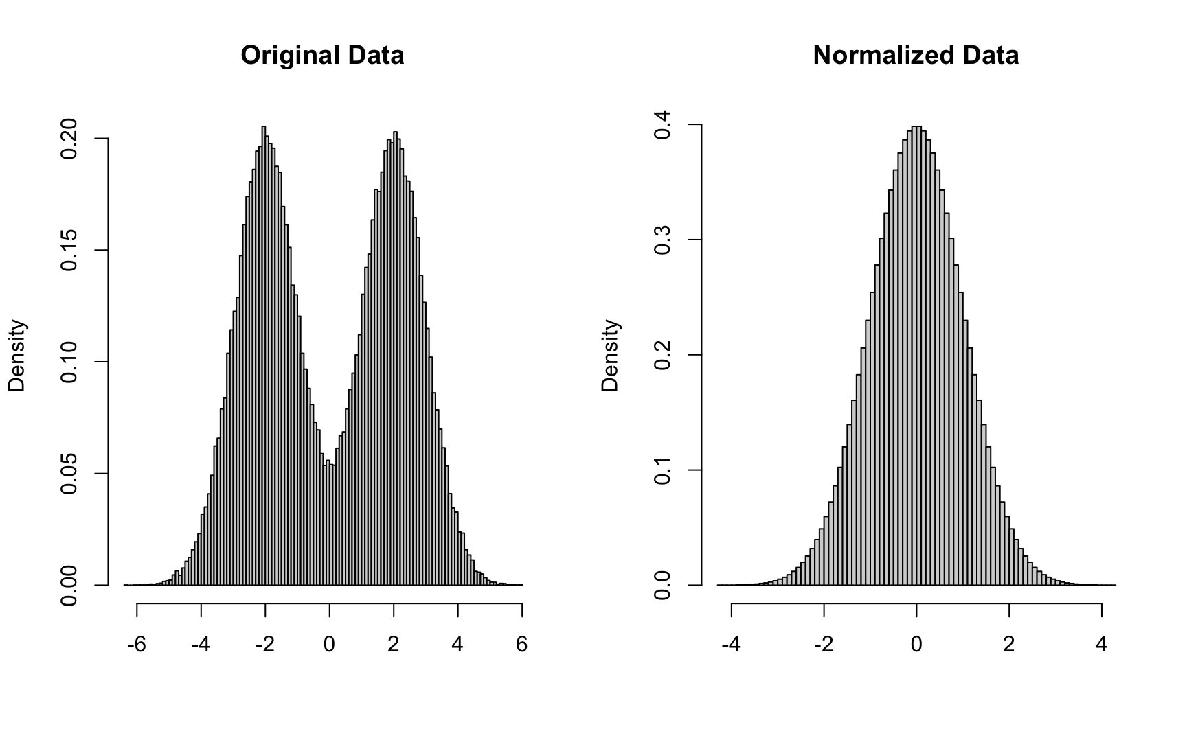
Figure 9.3: Comparsion between raw data and normalized data distribition
9.5.1.3 Step 4: ABC Posterior Simulation
Up to this point we have obtained all the information required for the the last part of the ABC algorithm, which is the estimation of the posterior functions. This step can be divided into 3 parts. The first part is to draw sample residual vectors from our previously defined residuals. We defined the residuals as a matrix named the Eps where each row of entry represents a sample. Thus we will randomly select n number of rows from Eps. The next part is to add each of these residuals to the regression prediction using \(Z_{obs}\) we obtained from the observed summary statistics \(\hat{\tau}_{obs}\) in previous steps. The last step is to convert the corresponding sample back to the original basis \(\tau\). This can be achieved by applying the reverse unconstrained and normalizing transformations. 9.4 shows our estimated posterior distribution for each \(\tau\) value.
n_post <- 1e5 # number of posterior ABC samples to draw
Eps_post <- Eps[sample(n_train, n_post, replace = TRUE),] # resample rows of Eps
# unconstrain tauhat_obs
X_obs <- logit(tauhat_obs, min = tauhat_rng[1], max = tauhat_rng[2])
# normalize X_obs
Z_obs <- sapply(1:ncol(X), function(ii) {
  norm_trans(X_obs[ii], xdata = X[,ii])
})
# add prediction to residual draws
mu_post <- c(Z_obs %*% Betahat) # predicted mean for each regression
# add to each colun of Eps_post
psi_post <- sweep(Eps_post, 2, STATS = mu_post, FUN = "+")
# inverse of normalizing transformation
theta_post <- sapply(1:ncol(theta), function(ii) {
  norm_itrans(psi_post[,ii], xdata = theta[,ii])
})
# inverse of unconstraining transformation
tau_post <- tau_cons(theta_post)

#+ reg_plot
tau_names <- c("tau[00]", "tau[11]", "tau[12]")
par(mfrow = c(1,3))
for(ii in 1:n_tau) {
  hist(tau_post[,ii], main = parse(text = tau_names[ii]),
       # posteriors are quite skewed, so zoom in on important part
       xlim = quantile(tau_post[,ii], probs = c(.01, .99)),
       breaks = 100, freq = FALSE)
  abline(v = tau_true[ii], col = "red")
}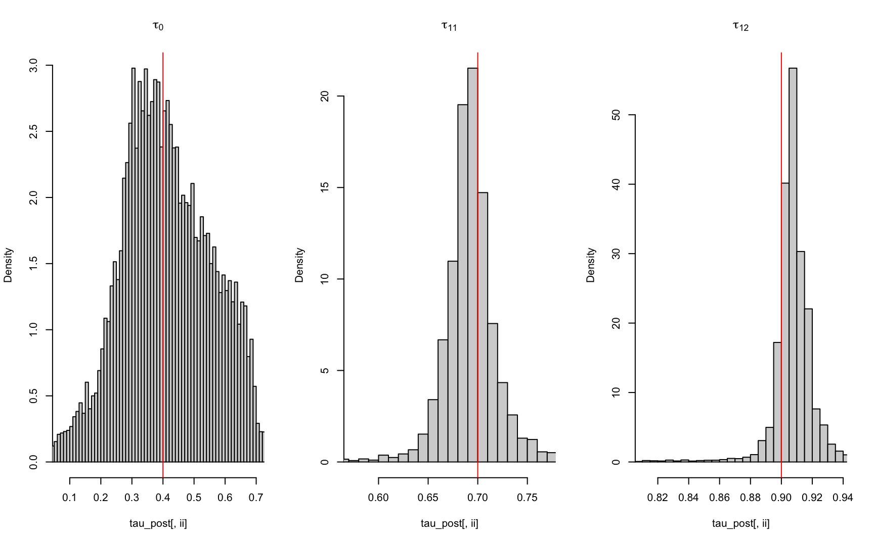
Figure 9.4: Estimated tau posterior distribution using ABC
Step 5: Generating True Posterior Distribution and Comparison
And finally we can generate the true posterior distribution and compare our accuracy. Please note that the actual ground truth for a 2-level NAC model cannot be obtained, the resulting posterior p(tau | U) cannot be sampled directly and evaluation of it is very expensive, such that MCMC would be extremely time-consuming. Instead, we’ll use a mode-quadrature normal approximation. Please note that since the focus of this chapter is not on the theory of mode-quadrature normal approximation only the high level-outline will be listed below. Readers are encouraged but not required to read additional material to better familiarize with the concept. For our demonstration purposes user can simply pretend the graph generated using code below is the actual posterior distribution of our 2-level NAC example.
#' 1.  First, we'll apply the mode-quadrature approximation to the unconstrained parameters `p(theta | U)` instead of `p(tau | U)`, as things always work better in an unconstrained basis.  Since the prior distribution is
#' ```
#' tau_tilde_00, tau_11, tau_12 ~iid Unif(0,1)
#' ```
#' where `tau_tilde_00 = tau_00 / min(tau_11, tau_12)`, by change-of-variables the corresponding prior on `theta = (theta_00, theta_11, theta_12)` becomes
#' ```
#' theta_00, theta_11, theta_12 ~iid f(theta),   f(theta) = exp(theta)/(1 + exp(theta))^2.
#' ```
#' 2.  Create a function equal to the log-posterior `log p(theta | U) = log p(U | theta) + log pi(theta)`, find the maximum `theta_hat` and the variance estimate
#'
#' ```
#' Sigma_hat = [-hessian( log p(theta_hat | U) )]^{-1}`.
#' ```
#' 4.  Approximately simulate `theta` from the posterior distribution by sampling from a multivariate normal with mean `theta_hat` and variance `Sigma_hat`.
#'
#'     **NOTE:** This isn't the exact posterior, but "mode-quadrature" approximation is probably a really good one, especially on the unconstrained parameter space of `theta`.  Also, this will be a lot faster than performing MCMC to sample from the exact posterior.
#' 5.  Convert `theta` back to `tau` by inverting the unconstraining transformation.
Below shows the actual comparison of the ABC posterior and the “exact” posterior, shown in figure 9.5
nac_nlp <- function(theta) {
  # convert to theta0 and theta1 as required inputs to dClaytonNAC
  tau <- tau_cons(theta)
  psi <- copClayton@iTau(tau)
  # loglikelihood
  ll <- sum(dClaytonNAC(U_obs, d = c(d_11, d_12),
                        theta0 = psi[1], theta1 = psi[2:3], log = TRUE))
  lpi <- sum(theta - 2 * log(exp(theta) + 1)) # log prior
  -(ll + lpi) # add log-prior
}

# calculate posterior mode
d_11 <- 5 # dimension of first NAC block
d_12 <- 15 # dimension of second NAC block
system.time({
  opt <- optim(par = c(0,0,0), fn = nac_nlp)
})
## user system elapsed
## 18.212 0.073 18.322# graphical check of solution
theta_hat <- opt$par # candidate mode
# projection plots
optimCheck::optim_proj(xsol = theta_hat,
fun = nac_nlp, maximize = FALSE)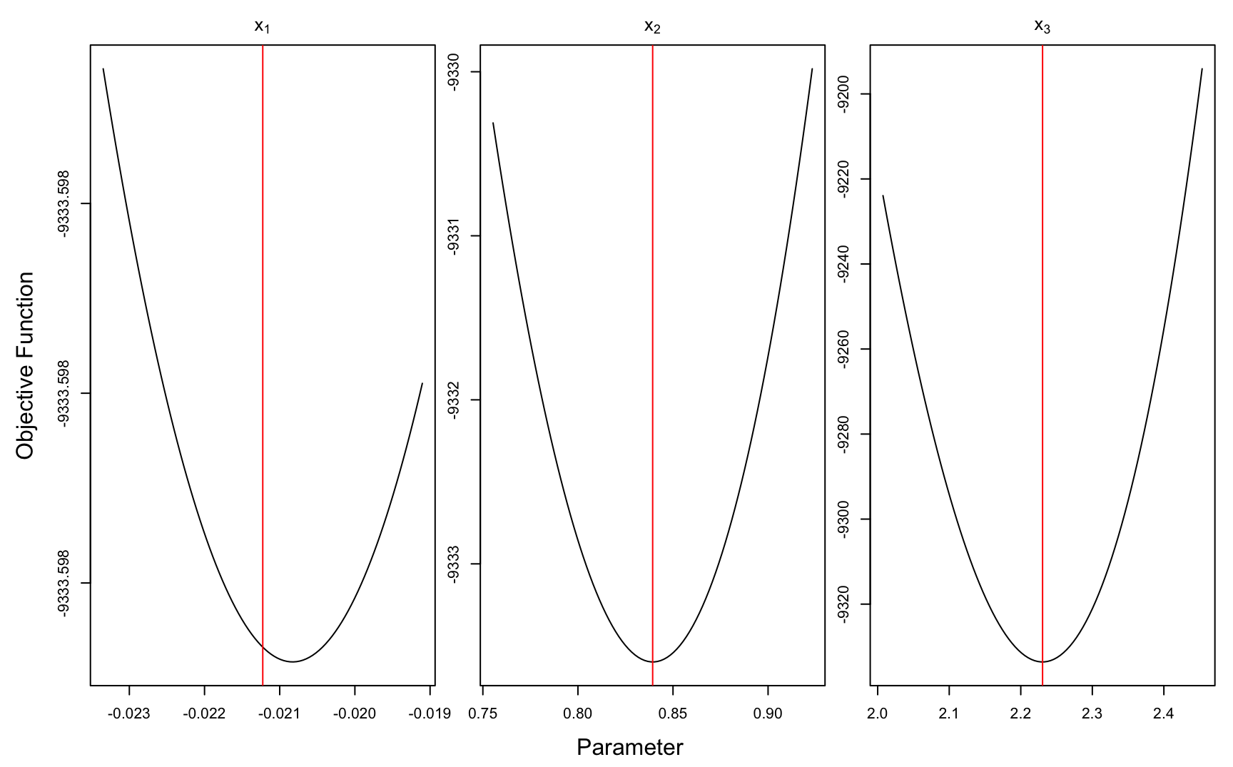
Figure 9.5: ‘Exact’ tau parameter distribution
# variance estimator
hess_hat <- hessian(nac_nlp, theta_hat) # quadrature
# check that it's positive definite
eigen(hess_hat)
## eigen() decomposition
## $values
## [1] 4968.91067 979.31402 48.68226
##
## $vectors
## [,1] [,2] [,3]
## [1,] -0.0001876797 -0.024908332 0.9996897218
## [2,] -0.0005569950 -0.999689582 -0.0249084327
## [3,] 0.9999998273 -0.000561497 0.0001737476Sigma_hat <- chol2inv(chol(hess_hat)) # stable matrix inverse for spd matrices
# sample from normal approximation to p(theta | U)
theta_mq <- mvtnorm::rmvnorm(n_post, mean = theta_hat, sigma = Sigma_hat)
# convert to p(tau | U)
tau_mq <- tau_cons(theta_mq)
# compare to abc approximation
tau_abc <- tau_postFigure 9.6 below shows the posterior distribution comparsion ABC, mode-quadrature and true tau values. Although the exact distribution graph is slightly off but the estiamted values are very alike. This shows that our code works in a complicated 2-level NAC models.
#+ comp_plot
tau_names <- c("tau[00]", "tau[11]", "tau[12]")
par(mfrow = c(1,3))
for(ii in 1:n_tau) {
  mq_dens <- density(tau_mq[,ii])
  abc_dens <- density(tau_abc[,ii])
  plot(abc_dens, type = "l", lwd = 2,
       ylim = range(mq_dens$y, abc_dens$y),
       xlim = range(mq_dens$x, quantile(tau_abc[,ii], probs = c(.01, .99))),
       main = parse(text = tau_names[ii]), ylab = "Density", xlab = "")
  lines(mq_dens, col = "blue", lwd = 2)
  abline(v = tau_true[ii], col = "red", lwd = 2)
  if(ii == 3) {
    legend("topleft",
           legend = c("Mode-Quadrature", "ABC", "True Tau"),
           fill = c("blue", "black", "red"))
  }
}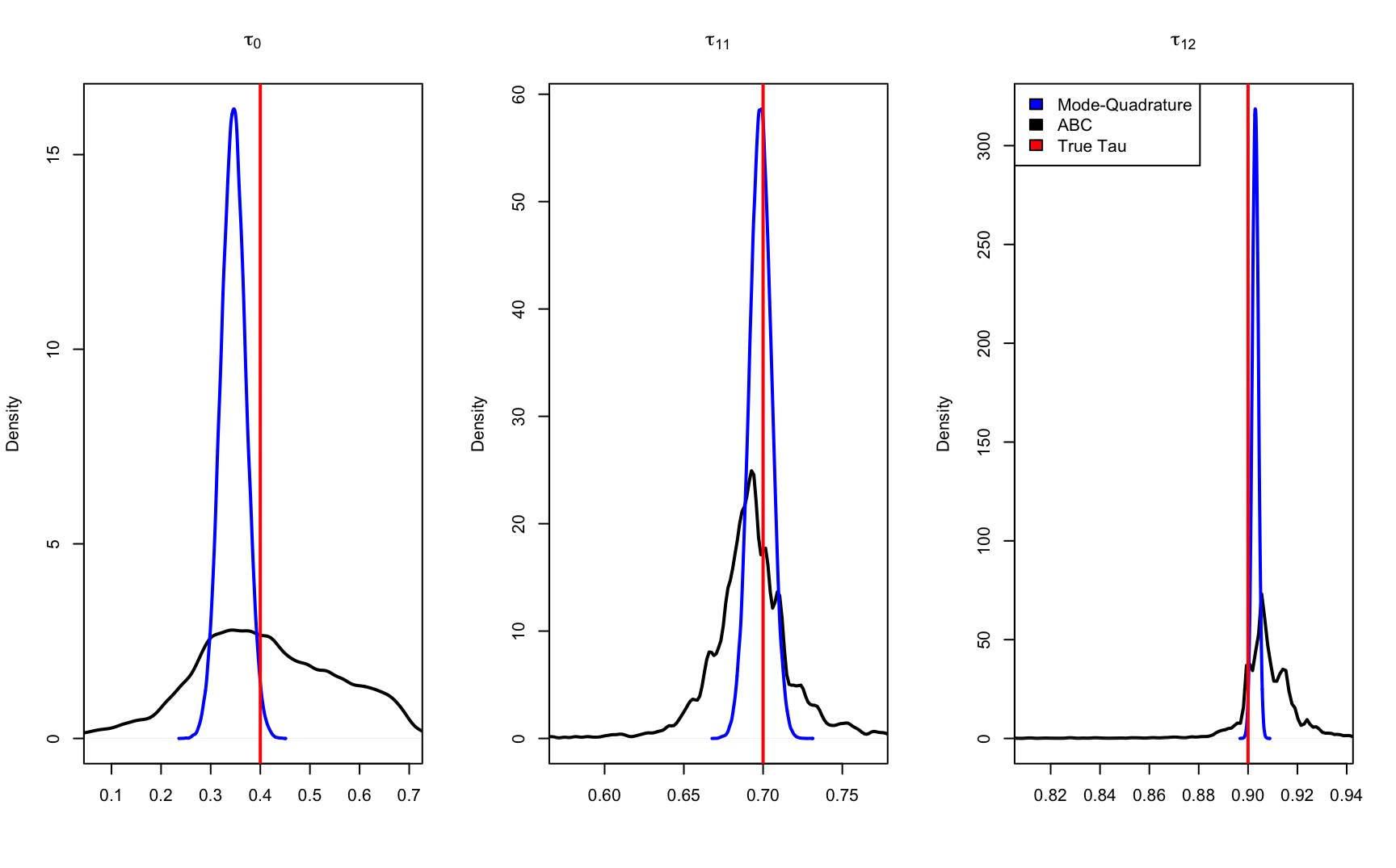
Figure 9.6: posterior distribution comparsion
9.6 APPENDIX A: R CODE
Helper functions used inside ABC algorithm Code from nacop-functions.R file
#--- abc helper functions ------------------------------------------------------

require(copula) # for NAC models
require(pcaPP) # for empirical Kendall's tau
require(partitions) # for `blockparts` to calculate NAC loglikelihood

#' Logit and inverse-logit transformations
#'
#' @param x Numeric argument.
#' @return Numeric of the same dimension as `x` computing its logit or inverse-logit.
logit <- function(x, min = 0, max = 1) {
  x <- (x - min)/(max - min)
  log(x) - log(1 - x)
}
ilogit <- function (x, min = 0, max = 1) {
  1/(1 + exp(-x)) * (max - min) + min
}

#' Convert `tau` to unconstrained basis.
#'
#' @param tau Vector of length 3 or 3-column matrix with elements (or columns) corresponding to `(tau_00, tau_11, tau_12)`.
#' @return Unconstrained transformation `(theta_00, theta_11, theta_12)` (see 'Details').
#' @details The parameter restrictions are `0 < tau_1i < 1` for `i = 1,2` and `0 < tau_00 < min(tau_11, tau_12)`.  Therefore, the unconstraining transformation is given by
#' ```
#' theta_1i = logit(tau_1i), i = 1,2
#' theta_00 = logit(tau_00 / min(tau_11, tau_12))
#' ```
tau_uncons <- function(tau) {
  if(!is.matrix(tau)) tau <- t(tau)
  ttau <- tau
  ttau[,1] <- tau[,1]/pmin(tau[,2], tau[,3])
  drop(logit(ttau))
}

#' Inverse of `tau_uncons`.
#'
#' Converts unconstrained `theta` back to `tau`.
#'
#' @param theta Vector of length 3 or 3-column matrix with elements (or columns) corresponding to `(theta_00, theta_11, theta_12)`.
tau_cons <- function(theta) {
  if(!is.matrix(theta)) theta <- t(theta)
  ttau <- ilogit(theta)
  tau <- ttau
  tau[,1] <- ttau[,1] * pmin(tau[,2],tau[,3])
  drop(tau)
}

#' Transform input to quantiles of the standard normal.
#'
#' @param x Vector of values to transform.
#' @param xdata Vector of values from which to compute the empirical CDF.
#'
#' @return Map of the rank of each `x` in `xdata` to the corresponding quantile of a `N(0,1)`.
norm_trans <- function(x, xdata = x) {
  ## rnk <- sapply(x, function(xi) sum(xi <= xdata))/(length(xdata)+1)
  N <- length(xdata)
  pct <- ecdf(xdata)(x) * N/(N+1) # ecdf correction to avoid 0 and 1
  qnorm(pct)
}

#' Inverse of `norm_trans()`.
#'
#' @param z Vector of normal quantiles.
#' @template param-xdata
#'
#' @return Maps each `z` to the corresponding quantile of `xdata`.
norm_itrans <- function(z, xdata) {
  quantile(xdata, prob = pnorm(z), names = FALSE)
}

#--- Analytic log-likelihood for 2-level Clayton-NACs --------------------------

require(copula) # simulate from NAC model
require(partitions) # for exact NAC likelihood
require(pcaPP) # for fast Kendall's tau

#' Simulate iid vectors from a Nested Archimedean Copula (NAC) distribution.
#'
#' @param n_obs Number of iid vectors to generate.
#' @param d_11 Dimension of the first block.
#' @param d_12 Dimension of the second block.
#' @param tau_00 Outer-level dependence parameter.
#' @param tau_11 Inner-level first block dependence parameter.
#' @param tau_12 Inner-level second block dependence parameter.
#' @param copfam String specifying the copula family.
#'
#' @return A matrix of size `n_obs x (d_11 + d_12)` of iid vectors from the NAC distribution.
sim_nac <- function(n_obs, d_11, d_12, tau_00, tau_11, tau_12, copfam) {
  # convert copula parameters from tau to theta
  theta <- iTau(getAcop(copfam), tau=c(tau_00, tau_11, tau_12))
  # construct NAC distribution object
  nac_list <- list(theta[1], NULL,
                   list(list(theta[2], 1:d_11),
                        list(theta[3], (d_11+1):(d_11+d_12))))
  cop_dist <- onacopulaL(family = copfam, nacList = nac_list)
  rCopula(n_obs, copula = cop_dist)
}

#' Simulate ABC training data.
#'
#' @param n_train Number of training samples.
#' @param n_obs Number of data observations.
#' @param d_11 Dimension of first inner block.
#' @param d_12 Dimensions of second inner block.
#' @details The prior on tau is:
#' ```
#' tau_11, tau_12 ~ind Unif(0,1)
#' tau_00 | tau_11, tau_12 ~ Unif(0, min(tau_11, tau_12))
#' ```
#' @return A data frame with `n_obs * (d_11 + d_12) + 3` columns corresponding to `(vec(U_train), tau_train)`, and approximately `n_train` rows, i.e., rejecting the bad samples.
sim_nac_train <- function(n_train, n_obs, d_11, d_12) {
  # generate tau
  tau_train <- cbind(tau_00 = runif(n_train),
                     tau_11 = runif(n_train),
                     tau_12 = runif(n_train))
  tau_train[,1] <- tau_train[,1] * pmin(tau_train[,2], tau_train[,3])
  # generate U | tau
  U_train <- lapply(1:n_train, function(ii) {
    sim_nac(n_obs = n_obs, d_11 = d_11, d_12 = d_12,
            tau_00 = tau_train[ii,1], tau_11 = tau_train[ii,2],
            tau_12 = tau_train[ii,3], copfam = "Clayton")
  })
  # eliminate bad samples
  bad_id <- sapply(U_train, anyNA)
  U_train <- U_train[!bad_id]
  tau_train <- tau_train[!bad_id,]
  # convert to data frame
  # names for elements of U: U_{ij} gets names "U_i_j"
  U_names <- expand.grid(1:n_obs, 1:(d_11 + d_12))
  U_names <- paste0("U_", U_names[[1]], "_", U_names[[2]])
  data_train <- do.call(rbind, lapply(U_train, c))
  data_train <- cbind(data_train, tau_train)
  colnames(data_train) <- c(U_names, "tau_00", "tau_11", "tau_12")
  data.frame(data_train)
}

#' Calculate Kendall's tau (sample version) for each pair of columns in a matrix.
#'
#' @param U Data matrix.  Each element should be between 0 and 1.
#' @param col_pairs Two row matrix where each column is a pair of columns from `U`.  If missing defaults to all `ncol(U) choose 2` unique pairs.
kendall_tau <- function(U, col_pairs) {
  if(missing(col_pairs)) {
  col_pairs <- combn(ncol(U), 2) # {d choose 2} pairs of columns
  }
  tau_hat <- apply(col_pairs, 2, function(ii) {
    cor.fk(U[,ii[1]], U[,ii[2]])
  })
  names(tau_hat) <- paste0("tau_hat_", col_pairs[1,], "_", col_pairs[2,])
  tau_hat
}


#' Density of 2-level Clayton NAC.
#'
#' @param u Matrix with `sum(d)` columns, where each row is an observation.
#' @param d Vector of integers specifying the size of each child copula, and for which `d0 = length(d)` is the size of the root copula.
#' @param theta0 Parameter of root copula (scalar).
#' @param theta1 Parameters of each child copula (vector of length `d0`).
#'
#' @return Vector `nrow(u)` densities.
dClaytonNAC <- function(u, d, theta0, theta1, log = FALSE) {
  d0 <- length(d)
  D <- sum(d)
  tu <- tcoeff(u, d = d, theta0 = theta0, theta1 = theta1)
  cu <- 0
  x <- matrix(NA, nrow(u), length(d0:D))
  for(kk in d0:D) {
    k2 <- kk-d0+1
    x[,k2] <- bcoeff(tu[,1:d0,drop=FALSE], k = kk, d = d,
                     theta0 = theta0, theta1 = theta1, log_abs = TRUE)
    x[,k2] <- x[,k2] - (kk+1/theta0) * log(1 + tu[,d0+1])
    x[,k2] <- x[,k2] + sum(log(abs(-1/theta0 - 1:kk + 1)))
  }
  ## xmax <- apply(x, 1, max)
  ## cu <- xmax + log(rowSums(exp(x - xmax)))
  cu <- logsumexp(x)
  cu <- cu + sum(d * log(theta1))
  lu <- log(u)
  s0 <- 0
  for(ss in 1:d0) {
    tmp <- (1+theta1[ss]) * rowSums(lu[,s0+1:d[ss],drop=FALSE])
    cu <- cu - tmp
    s0 <- s0 + d[ss]
  }
  if(!log) cu <- exp(cu)
  cu
}

#' Construct the `outer_copula` object for a 2-level Clayton NAC.
#'
#' @param d Vector of integers specifying the size of each child copula, and for which `d0 = length(d)` is the size of the root copula.
#' @param theta0 Parameter of root copula (scalar).
#' @param theta1 Parameters of each child copula (vector of length `d0`).
#'
#' @return An object of type `outer_copula`.
ClaytonNAC <- function(d, theta0, theta1) {
  d0 <- length(d)
  l2 <- NULL # level 2
  s0 <- 0
  for(ss in 1:d0) {
    l2 <- c(l2, list(list(theta1[ss], s0 + 1:d[ss])))
    s0 <- s0 + d[ss]
  }
  onacopulaL(family = "Clayton", nacList = list(theta0, NULL, l2))
}

pClaytonNAC <- function(u, d, theta0, theta1) {
  cop <- ClaytonNAC(d, theta0 = theta0, theta1 = theta1)
  pCopula(u, copula = cop)
}

rClaytonNAC <- function(n, d, theta0, theta1) {
  cop <- ClaytonNAC(d, theta0 = theta0, theta1 = theta1)
  rCopula(n, copula = cop)
}

#' Calculates `(-1)^n`
parity <- function(n) {
  -2 * (n %% 2) + 1
}

#' Calculates the falling factorial `(x)_n`.
fallfac <- function(x, n) {
  xn <- x - (1:n) + 1
  parity(sum(sign(xn) < 0)) * exp(sum(log(abs(xn))))
}

#' Calculates `Q_{d,k}`.
#' @param d Vector of integers.
#' @param k Integer index value.
Qcoeff <- function(d, k) {
  d0 <- length(d)
  blockparts(d - rep(1L, d0), k-d0) + 1
}

#' Calculates `a_{nk}(t)` for 2-level Clayton NACs.
#'
#' @param t Vector of nonnegative reals.
#' @param n Integer index.
#' @param k Vector of integers between `1` and `n`.
#' @param theta0,thetas Root and child generator parameters (scalars).
#' @param log_abs If `TRUE` returns `log(abs(a_{nk}(t)))`.
#'
#' @return A matrix of size `length(t) x length(k)`.
#'
acoeff <- function(t, n, k, theta0, thetas, log_abs = FALSE) {
  alphas <- theta0/thetas
  lsnk <- coeffG(d = n, alpha = alphas, log = TRUE)[k]
  lac <- outer(log(1+t), alphas*k - n, FUN = "*")
  lank <- sweep(lac, 2, lsnk, FUN = "+")
  if(!log_abs) lank <- sweep(exp(lank), 2, parity(n - k), FUN = "*")
  lank
  ## snk <- parity(n - k) * coeffG(d = n, alpha = alphas)[k]
  ## ac <- exp(outer(log(1+t), alphas*k - n, FUN = "*"))
  ## sweep(ac, 2, snk, "*")
}

#' Calculates `b_{dk}(t)` for 2-level Clayton NACs.
#'
#' @param t Matrix of nonnegative reals with `d0 = length(d)` columns.
#' @param k Integer index of function.
#' @param d,theta0,theta1 See `dClaytonNAC()`.
#' @param log_abs If `TRUE` calculates `log(abs(b_{dk}(t)))`.
bcoeff <- function(t, k, d, theta0, theta1, log_abs = FALSE) {
  d0 <- length(d)
  Qdk <- Qcoeff(d = d, k = k)
  nQ <- ncol(Qdk)
  nt <- nrow(t)
  # calculate only the necessary lAnk = log(abs(Ank))
  # also label the columns to easily extract with Qdk
  K <- lapply(1:d0, function(ss) unique(Qdk[ss,]))
  nK <- sapply(K, length)
  lAnk <- matrix(NA, nt, sum(nK))
  colnames(lAnk) <- rep(NA, ncol(lAnk))
  Rdk <- matrix(NA, d0, nQ)
  s0 <- 0
  for(ss in 1:d0) {
    lAnk[,s0+1:nK[ss]] <- acoeff(t[,ss], n = d[ss], k = K[[ss]],
                                 theta0 = theta0, thetas = theta1[ss],
                                 log_abs = TRUE)
    colnames(lAnk)[s0+1:nK[ss]] <- paste0(ss, "_", K[[ss]])
    Rdk[ss,] <- paste0(ss, "_", Qdk[ss,])
    s0 <- s0 + nK[ss]
  }
  lbdk <- matrix(NA, nt, nQ)
  for(jj in 1:ncol(Qdk)) {
    lbdk[,jj] <- rowSums(lAnk[,Rdk[,jj],drop=FALSE])
  }
  lbdk <- logsumexp(lbdk)
  if(!log_abs) lbdk <- parity(sum(d)-k) * exp(lbdk)
  lbdk
  ## bdk <- matrix(NA, nt, nQ)
  ## for(jj in 1:ncol(Qdk)) {
  ##   bdk[,jj] <- apply(Ank[,Rdk[,jj],drop=FALSE], 1, prod)
  ## }
  ## rowSums(bdk)
}

#' Calculate `t(u)` for the 2-level Clayton NAC.
#'
#' @param u,d,theta0,theta1 See `dClaythonNAC()`.
#'
#' @return A matrix with `length(d) + 1` columns, the first `d0 = length(d)` of which are `t_s(u_s)`, and the last of which is `t(u)`.
tcoeff <- function(u, d, theta0, theta1) {
  d0 <- length(d)
  tu <- matrix(NA, nrow(u), d0+1)
  Cu <- matrix(NA, nrow(u), d0)
  s0 <- 0
  for(ss in 1:d0) {
    tu[,ss] <- rowSums(u[,s0+1:d[ss],drop=FALSE]^(-theta1[ss]) - 1)
    Cu[,ss] <- (1 + tu[,ss])^(-1/theta1[ss])
    s0 <- s0 + d[ss]
  }
  tu[,d0+1] <- rowSums(Cu^(-theta0) - 1)
  tu
}

#' Calculate the log-sum-exp in each row of input.
#'
#' Calculates `log(abs(sum(sx[i,] * exp(x[i,]))))` for each row of `x`.
#'
#' @param x Vector or matrix.
#' @param sx Optional sign of `exp(x)`.  Default value is 1.
#' @param sgn If `TRUE` also returns the sign of `sum(sx[i,] * exp(x[i,]))`.
#'
#' @return A vector or two-column matrix if `sgn = TRUE`.
logsumexp <- function(x, sx, sgn = FALSE) {
  if(!is.matrix(x)) x <- t(x)
  if(missing(sx)) {
    sx <- matrix(1, nrow(x), ncol(x))
  } else {
    if(!is.matrix(sx)) sx <- t(sx)
  }
  # transpose inputs
  x <- t(x)
  sx <- t(sx)
  mx <- apply(x, 2, max)
  y <- colSums(sx * exp(sweep(x, 2, mx)))
  if(sgn) sy <- sign(y)
  y <- log(abs(y)) + mx
  if(sgn) y <- cbind(y, sy)
  y
}

#--- scratch -------------------------------------------------------------------