Chapter 6 Stochastic Differential Equations
6.1 Prerequisites
In this chapter we will introduce the stochastic differential equation (SDE). We will see that an SDE is an integral equation which can be thought of as the stochastic analogue of a differential equation. Unlike standard differential equations, the solution of an SDE is a stochastic process. Common applications of SDE include stock price modelling or tracing of thermal fluctuations in a physical system.
For the remainder of this chapter we will assume that every stochastic process takes its values in \(\mathbb{R}\) and has, as its domain, the ambient sample space \(\Omega\) equiped with a probability function \(P\). Unless stated otherwise, we assume that the stochastic process \(X_t\) is continuous time where \(t \in \mathbb{T} = [0, T]\). For the remainder of this module, it will be helpful to keep in mind that we may think of a stotchastic process \(X_t\) as a function of two variables, namely, \(t \in \mathbb{T}\) and \(\omega \in \Omega\). To emphasize this point some authors write \(X(t, \omega)\), where \(X(t, \cdot)\) is a random variable, and where \(X(\cdot, \omega)\) is a function from \(T\) to \(\mathbb{R}\), also called the sample path of the variable. From this one could just as well think of \(X_\cdot\) as a random variable which takes its values in the space of functions from \(T\) to \(\mathbb{R}\). Note that, since a random variable is, in essence, just a function we can truly think of our stochastic process \(X\) as any other function of two variables: \[ X: T \times \Omega \longrightarrow \mathbb{R} \] This means that there should be nothing particularily new in an expression like this: \[ \int X_t \: \ud t = \int X(t, \omega) \: \ud t \] or this: \[ \frac{\ud X_t}{\ud t} = \frac{\partial X}{\partial t}(t, \omega) \] or the statement “\(X_t\) is continunous with respect to \(t\)”. These are simply standard expresesions of multivariable calculus.
We will stick with the convention of writing the time argument as a subscript \(t\) and omitting the \(\omega\) argument when it is not necessary to include. This will make the notation more consistent with conventions in the general theory of probability and statistics. But keep in mind, whenever calculus is being done, it is helpful to think of \(X_t\) as a function of two variables.
There are two foundamental principals underlying SDE: Brownian motion and Markov process. In the next subsections, we discuss these two fundamental notions behind SDE.
6.1.1 Brownian Motion
The idea of Brownian motion came about in the year 1827 as botanist Robert Brown studied the motion of a pollen particle immersed in water. His observations were curious: The particles constantly jitter and erratically move in a seemingly random fashion. Robert Brown at first hypothesized that the pollen particle must be living, but later rejected the hypothesis after observing the same peculiar motion with inorganic substances. Puzzled by the phenomena, Brown states:
Extremely minute particles of solid matter, whether obtained from organic or inorganic substances, when suspended in pure water, or in some other aqueous fluids, exhibit motions for which I am unable to account…
It was only until 1905, that the true explination for what Robert Brown observed was provided by none other than Einstein himself. To simplify Einsten’s argument suppose that our pollen particle could only move in two dimensions, left or right. Einstein argued that at each unit of time the pollen particle was being bombarded by a countless number of tiny water molecules, which caused the motion of the pollen. Of course, relative to the water molecules, a particle of pollen is massive. Hence, each water molecule contributes only a tiny amount to the displacement of the water molecule. Suppose that:
- Our pollen particle gets hit by \(N\) water molecules per second
- Each water molecule hits in an equal interval of time
- Each water molecule contributes discplacement given by a random variable \(Z_i \sim N(0, \Delta t)\) where \(\Delta t = 1/N\).
If \(B_t\) represents the position of our pollen particle then total displacement at the end of one second is given by: \[ B_1 = B_0 + \sum_{i = 1}^N Z_i \] Where \(B_0\) is a fixed, non-random initial position. Being the sum of iid normal random variables, it follows that \(B_1 \sim N(B_0, 1)\). For each intermediate unit of time \(t \in [0, 1]\) the displacement is given by: \[ B_t = B_0 + \sum_{i = 1}^{\lfloor {tN} \rfloor} Z_i \] Where \(\lfloor \cdot \rfloor\) returns the nearest integer rounded down from the argument. Note that \(\lfloor tN \rfloor = n\) for some \(n = 0, 1, \dots, N -1, N\), where \(\sum_{i=1}^0 Z_i = 0\). Hence, for \(n\) satisfying the above we may equivalently write:
\[ B_t = B_{n \Delta t} = B_0 + \sum_{i = 1}^{n} Z_i \]
But since the above formula imples our particle of pollen is instentanously moving from point to point, we correct for this by a process of linear interpolation, i.e. by drawing a straight line from \(B_{n \Delta t}\) to \(B_{(n + 1) \Delta t}\) to obtain a continuous process. Brownian motion proper, is, in a certain sense, simply the limit of the above process as \(N \longrightarrow \infty\).
Of course, there is no particular reason that our process should take place only for 1 second. We can extend our unit of time to encompase any interval \([0, T]\) by rescaling \(\Delta t = T/N\).
The above remarks should motivate the formal definition of Brownian motion, as well as our later discussion of how to simulate the process with discrete time intervals.
Definition: Brownian motion (\(B_t\), also called Wiener process when \(B_1 \sim N(0, 1)\)) is a continuous-time stochastic process with the following properties:
Almost every sample path of \(B\) is continuous (i.e. \(P(\{\omega: B_t(\omega) \text{ is continous in t} \}) = 1\)).
\(B_t\) has independent increments. Think of the index \(t\) as time. If \(t_0<t_1<...<t_N\), then Brownian Motion increments of non-overlapping time intervals are independent, that is, \[ B_{t_1}-B_{t_0} \perp\!\!\!\perp B_{t_2}-B_{t_1} \perp\!\!\!\perp \ ... \perp\!\!\!\perp B_{t_N}-B_{t_{N-1}}\]
\(B_{t}\) is a Gaussian process, where \(B_{s+t}-B_{s} \sim \mathcal{N}(0,t)\).
It is also a common practice to assume \(B_0 = 0\), but this is not a requirement.
Brownian motion is often used in physical sciences to study diffusion processes, quantum mechanics, or cosmology (e.g.black-holes). It is also used in the mathemetical theory of finance to model the stock option pricing.
Simulating Brownian motion is relatively simple and follows immediately from our earlier discussion. To simulate \(B_t\) on \([0,T]\) at intervals of \(\Delta t=T/N\):
Set \(B_0\)
Draw \(Z_1,...Z_N \overset{\text{iid}}{\sim} \mathcal{N}(0,\Delta t)\)
Let \(B_{n\Delta t} = B_0 + \sum_{i=1}^{n}Z_i\)
<Fig 1> shows the traces of Brownian motions for \(t=1,...,2000\), where \(B_{s+1}-B_{s} \sim \mathcal{N}(0,1) \ \forall s\). Each traces (depicted by different colors) represent the trace of this Brownian motion with a different \(B_0\). R code to generate <Fig 1> is found in Section 1.3.
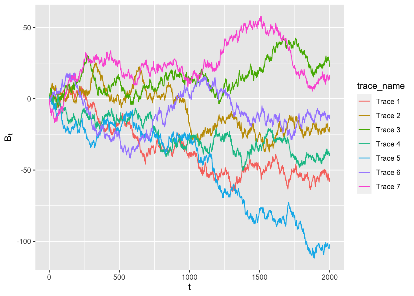
<Fig 1: Traces of Brownian motions for \(t = 1,...,2000\), where \(B_{s+1}-B_{s} \sim \mathcal{N}(0,1) \ \forall s\)>
6.1.2 Markov Processes
Definition: A Markov chain is a stochastic process that is used to model a sequence of events in which the probability of the current event (\(X_t\)) is only dependent on the event that is immidiately previous to the current one (\(X_{t-1}\)). If a Markov chain process is continuous-time (\(X_t\) is continuous in \(t\)), it is called a Markov process and is defined by the following two properties:
almost every sample path of \(X_t\) is continuous
\(X_t\) has the homogeneous Markov property:
\[ Pr(X_{t+s}|{X_u=x_u: u \leq t}) = Pr(X_{t+s}|X_t=x_t) = Pr(X_s|X_0=x_t) \]
Markov chains have many applications as statistical models of real-world processes, such as studying cruise control systems in motor vehicles, queues or lines of customers arriving at an airport, currency exchange rates and animal population dynamics.
6.2 R Code for Section 1
This section provides the R code used to generate the figures in the previous section.
6.2.1 Code to simulate the Brownian motion (<Fig 1>)
library(ggplot2)

# define the maximum value for the time (=2000)
t_max <- 2000
# specify the number of Brownian motion graphs that will be drawn on a window
n_graph <- 7
# make a data frame to store the B_t's
df_B <- data.frame(matrix(nrow = t_max*n_graph, ncol=1))

# randomly draw 2000 values from the standard normal distribution (mean=0, var=1),
# and store the results as norm_vec.
# setting the var=1 implies that our time increment (delta-t) is equal to 1.
# the first element of norm_vec is the B_0
# the second element of norm_vec is B_1-B_0, the third element of norm_vec is B_2-B_1,...
for (i in c(1:n_graph)){
  norm_vec <- rnorm(t_max,0,1)
  B_t <- cumsum(norm_vec)
  B_t <- B_t - B_t[1]
  df_B[(1+(i-1)*t_max):(i*t_max),] <- B_t
}

# to make a ggplot of Brownian motion graphs,
# our data frame has to have a column that specifies which observation belongs to which trace.
# make a data frame column trace_name for this purpose
trace_name <- data.frame(c(rep("Trace 1",t_max), rep("Trace 2", t_max),
                           rep("Trace 3", t_max), rep("Trace 4", t_max),
                           rep("Trace 5", t_max), rep("Trace 6", t_max),
                           rep("Trace 7", t_max)))

# make a data frame column that specifies the value for the time variable
time <- data.frame(rep(c(1:t_max),n_graph))

# add the new data frame columns that we made onto the existing data frame, to make a ggplot
df <- data.frame(cbind(trace_name, time, df_B))
colnames(df) <- c("trace_name","time","df_B")

# make a ggplot object
ggplot(df, aes(x=time, y=df_B ,group=trace_name, color=trace_name)) + geom_line() + xlab(expression("t")) + ylab(expression("B"[t]))
6.3 Stochastic Differential Equation
In this section, we provide the basic definition of the stochastic differential equation (SDE). We also describe the Euler approximation algorithm which will be used in Section 3 (computational examples of SDE).
6.3.1 Definition
A stochastic differential equation (SDE) is defined from the Brownian motion (Section 1.1) and Markov process (Section 1.2). More specifically, let \(X_t\) be a stochastic process such that all of the followings hold:
\(X_t\) is a continuous process in \(t\)
\(X_t\) has the homogeneous Markov property \[Pr(X_{t+s}|{X_u=x_u: u \leq t}) = Pr(X_{t+s}|X_t=x_t) = Pr(X_s|X_0=x_t)\]
Then, up to a mathematical sigularity, \(X_t\) is a diffusion process which can be expressed as a stochastic differential equation as below: \[\ud X_t = \mu(X_t) \ud t+\sigma(X_t) \ud B_t,\]
where \(\mu(x)\) and \(\sigma(x)\) are the drift and diffusion functions respectively, and \(B_t\) is a Brownian motion.
Think of \(\ud X_t\) as the net change in \(X\) at time \(t\), and \(\mu(X_t)\) as the average rate of change in \(X\) at time \(t\) (\(E(\frac{\ud X}{\ud t})\) at time \(t\)). Also take \(\sigma(X_t)\) as the rate of variation in \(X\) with respect to \(B\) at time \(t\) (\(\frac{\ud X}{\ud B}\) at time \(t\)). Then the stochastic differential equation above can be interpreted as:
(net change in \(X\) at time \(t\)) \(=\)
(average amount of change in \(X\) at time \(t\)) \(+\) (variation in the amount of change in \(X\) at time \(t\)),
where:
(net change in \(X\) at time \(t\)) \(= \ud X_t\)
(average amount of change in \(X\) at time \(t\)) \(= \mu(X_t) \ud t\), and
(variation in the amount of change in \(X\) at time \(t\)) \(=\sigma(X_t) \ud B_t\)
Example 2.1: Let \(X_t\) be a diffusion process (i.e. \(X_t\) can be expressed as a stochastic differential equation \(\ud X_t = \mu(X_t) \ud t+\sigma(X_t) \ud B_t\)). If \(\ud X_t = \ud B_t\) and \(B_0=0\), then \[ \begin{align} X_t &= X_0 + (X_t-X_0) \\ &= X_0 + \int_{0}^{t} \ud X_s &&[X_t-X_0=\int_{0}^{t} \ud X_s] \\ &= X_0 + \int_{0}^{t} \ud B_s &&[\ud X_s=\ud B_s] \\ &=X_0+B_t &&[B_0=0]\\ \end{align} \] That is, \(X_t\) is a Brownian motion.
Example 2.2: Let \(X_t\) be a diffusion process. If \(\ud X_s = \mu \ud s+ \sigma \ud B_s\) and \(B_0 = 0\), then
\[ \begin{align} X_t &= X_0 + (X_t-X_0) \\ &= X_0 + \int_{0}^{t} \ud X_s \\ &= X_0 + \int_{0}^{t} (\mu \ud s+ \sigma \ud B_s) &&[\ud X_s=\mu \ud s+ \sigma \ud B_s] \\ &= X_0 + \int_{0}^{t} \mu \ud s+ \int_{0}^{t} \sigma \ud B_s \\ &=X_0+\mu t+\sigma B_t \;. \end{align} \]
That is, \(X_t\) is a brownian motion with a drift.
Example 2.3: Let \(B_t\) be a Brownian motion, and let \(X_t=g(B_t)\), where \(g\) is a monotonically increasing continuous function. Then, since both \(g\) and \(B_t\) are continuous, \(X_t\) must be continuous as well. Also,
\[ \begin{align} \Pr(X_{t+s} \leq x \mid {X_u=x_u: u \leq t}) &= \Pr(g(B_{t+s} \leq x \ | \ {g(B_u)=x_u:u\leq t})) &&[X_t=g(B_t)] \\ &= \Pr(B_{t+s} \leq g^{-1}(x) \ \mid \ {B_u=g^{-1}(x_u):u \leq t}) &&[\frac{\ud g}{\ud B} > 0, \forall B] \\ &= \Pr(B_{t+s} \leq g^{-1}(x) \ \mid \ B_t=g^{-1}(x_t)) &&[B_{t_2}-B_{t_1} \ \amalg \ \dots \ \amalg \: B_{t_n}-B_{t_{n-1}}] \\ &= \Pr(g(B_{t+s}) \leq x \ \mid \ g(B_t)=x_t) \\ &= \Pr(X_{t+s} \leq x \ \mid \ X_t=x_t) \\ \end{align} \]
so \(X_t\) also has the Markov property. Hence, \(X_t\) is a diffusion process. The fact that \(X_t\) is a diffusion process implies that \(X_t\) must be described by a SDE. It turns out that this SDE is:
\[ \ud X_t = \frac{1}{2}g{''}(g^{-1}(X_t)) \ \ud t + g'(g^{-1}(X_t)) \ \ud B_t \]
This is called Itô’s lemma. The Itô’s lemma section under the Appendix informally gives an insight into why the lemma works. The formal proof for the Itô’s lemma can be found here.
Example 2.4 (continuing from Example 2.3): In Example 2.3, we saw that \(X_t=g(B_t)\) is a diffusion process. How should we simulate a diffusion process \(X_t=x_0+g(B_t), B_0=0\) on \([0,T]\) at intervals of \(\Delta t = T/N\)? We can use the algorithm below:
Draw \(Z_1,...,Z_n \iid \N(0,\Delta t)\).
Recall that by the definition of Brownion motion, \(B_{t+\Delta t}-B_{t} \sim \N(0,\Delta t)\).
Hence, \(Z_1,...,Z_n\) represent increment in \(B\) at each consecutive time interval of length \(\Delta t = T/n\).Let \(B_{n\Delta t} = \sum^{n}_{i=1}Z_i\).
Since \(B_0=0\) and \(Z_i=\)(increment in \(B\) at the \(i^{th}\)) time interval, \(\sum^{n}_{i=1}Z_i=0+Z_1+Z_2+...+Z_n=\) (value of \(B\) at time \(t=n \Delta t\) ) \(=B_{n\Delta t}\).Let \(X_{n\Delta t} = x_0 + g(B_{n \Delta t})\).
6.3.2 Euler Approximation
As illustrated in Example 2.4, it is relatively easy to simulate \(X_t=x_0+g(B_t)\) because in this case \(X_t\) is in a relatively simple functional form of \(B_t\). However, it is often the case that \(X_t\) cannot be expressed in such a simple form involving \(B_t\). In general, \(Pr(X_t \ | \ X_0)\) is likely to be intractable, so we cannot always simulate the exact values of \(X_{\Delta t}, X_{2\Delta t},...\). This raises the need for an algorithm that would allows to simulate \(X_t\) approximately. A popular method for such an approximate simulation is the Euler approximation. The Euler approximation simulates the \(X_t\) on \(t \in [0,T]\) at intervals of length \(\Delta t = T/N\).
Euler approximation algorithm:
Consistent with the definition of Brownian motion, draw \(\Delta B_0,.., \Delta B_{N-1} \overset{\text{iid}}{\sim} \mathcal{N}(0,\Delta t)\),
where \(\Delta B_n = B_{(n+1)\Delta t}-B_{n \Delta t}\).Let \(\tilde{X_0}=x_0\).
Let \(\tilde{X}_{(n+1)\Delta t} = \tilde{X}_{n\Delta t} + \Delta\tilde{X}_{n} \approx \tilde{X}_{n\Delta t} + \mu(\tilde{X}_{n\Delta t})\Delta t+\sigma(\tilde{X}_{n\Delta t}) \Delta B_n\),
where \(\Delta\tilde{X}_{n} = \text{(change in } \tilde{X} \text{ during the } (n+1)^{th} \text{ time interval)} = \tilde{X}_{(n+1)\Delta t} - \tilde{X}_{n\Delta t} \approx \mu(\tilde{X}_{n\Delta t}) \Delta t+\sigma(\tilde{X}_{n\Delta t}) \Delta B_n\).
The Euler approximation method has a desirable property, namely:
if \(\tilde{X}_{t}^{(N)}\) is the Euler approximation of the \(X_t\) (\(t \in [0,T]\)) at intervals of length \(\Delta t = T/N\), we have
\[ \lim\limits_{N \to \infty}\sup\limits_{0 \leq t \leq T}E[(\tilde{X}_{t}^{(N)}-X_t)^2]=0 \]
In particular, \(\lim\limits_{N \to \infty}Pr(\tilde{X}_{t}^{(N)} \ | \ X_0)=Pr(X_t \ | \ X_0)\).
This desirable property of Euler approximation makes sense since as \(N \to \infty\) (i.e. as the length of the time interval gets infinitesimally small), \(\tilde{X}_{t}^{(N)}\) more closely resembles the original diffusion process \(X_t\) which is continuous in \(t\). Hence, the difference between \(\tilde{X}_{t}^{(N)}\) and \(X_t\) should reduce down to \(0\) as \(N \to \infty\). Example 2.5 below demonstrates this desirable property of the Eular approximation.
Example 2.5 (Demonstrating the desirable property of Eular approximation):
A Geometric Brownian Motion (GBM) is any continuous-time process in which the log of the randomly varying quantity is the Brownian motion. A stochastic process \(S_t\) is said to follow a GBM if the process can be described with the stochastic differential equation \(\ud S_t = \mu S_t \ud t+\sigma S_t \ud W_t\). GBM is the most widely used model for analyzing fluctuation in stock price.
We visualize the desirable property of the Euler approximation by plotting the density of a GBM for varying values of the parameter \(N\) (number of intervals in which to split \([t_0, T]\)). For this example, we pick \(S_t = x\exp\{(r-\frac{\sigma^2}{2}(0.3)^2)t+\sigma B_t\} = \exp\{(0.1-\frac{(0.3)^2}{2})t+(0.3)B_t\}\), where \(x=1, \ r=0.1, \ \sigma=0.3, \ T= 3.2\), for our GBM.
We know that this \(S_t\) is a GBM since this particular process is associated with the stochastic differential equation of the form \(\ud S_t = \mu S_t \ud t+\sigma S_t \ud W_t\). This can be derived by Itô’s integration (for interested readers, we provided a special section on the Itô’s integration under the Appendix). More details on how our \(S_t\) is associated with the stochastic differential equation can be found here.
<Fig 2> shows the plots of the (density from the Euler approximation of our GBM) vs. (the true density of our GBM), for the varying values of \(N\):
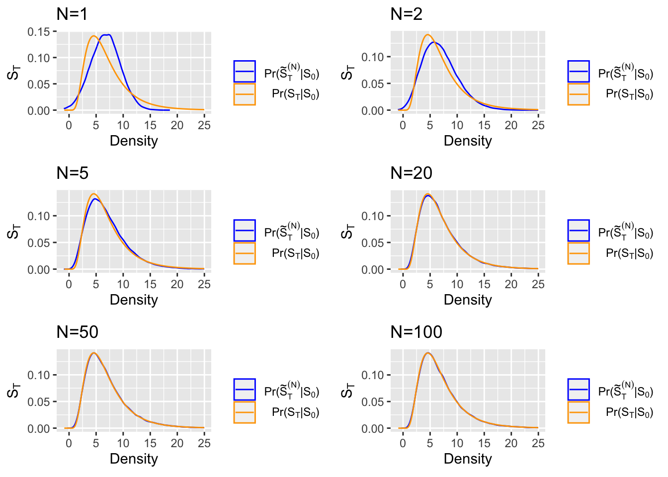
<Fig 2: Euler density vs. actual density of the GBM \(S_t = \exp\{(0.1-\frac{(0.3)^2}{2})t+(0.3)B_t\}\)>
6.4 R Code for Section 3
This section provides the R code used to generate the figures in Chapter 2.
6.4.1 Code to simulate the Brownian motion (<Fig 2>)
#' A function to calculate Euler approximations of a geometric Brownian motion.
#' @param n Number of random vectors (i.e., time series) to generate.
#' @param alpha Rate parameter of gBm.
#' @param sigma Volatility parameter of gBm.
#' @param dT Time between observations.
#' @param N Length of each time series.
#' @return An `N x n` matrix of iid time series, each of which is a column.
gbm.sim <- function(n, alpha, sigma, dT, s0, N) {
  SS <- matrix(NA, n, N+1) # always faster to fill matrix by column than by row
  SS[,1] <- s0 # initial value
  for(ii in 2:(N+1)) {
    dB <- rnorm(n, sd = sqrt(dT))
    SS[,ii] <- SS[,ii-1] + alpha*SS[,ii-1] * dT + sigma*SS[,ii-1] * dB
  }
  t(SS[,-1]) # customarily each column is a time series
}

#' A function to calculate the exact transition density of geometric Brownian motion.
#'
#' @param s Value(s) at which to evaluate `St`.
#' @param alpha Rate parameter of gBM.
#' @param sigma Volatility parameter of gBM.
#' @param t Time between `S0` and `St`.
#' @param s0 Initial value of process on which to condition.
#' @param log Logical; whether or not conditional PDF is returned on the log-scale.
#' @return Conditional PDF evaluation(s).
#' @details Geometric Brownian motion is a stochastic process \eqn{S_t} satisfying the stochastic differential equation (SDE)
#' \deqn{
#' d S_t = \alpha S_t dt + \sigma S_t dB_t.
#' }
dgbm <- function(s, alpha, sigma, s0, t, log = FALSE) {
  dlnorm(s, log = log,
         meanlog = (alpha - sigma^2/2)*t + log(S0),
         sdlog = sigma * sqrt(t))
}

# making ggplot of (actual density) vs. (Euler approximation density)
#
#
library(ggpubr)
library(ggplot2)

# simulation parameters
S0 <- 5.1 # initial value
alpha <- .1 # rate parameter
sigma <- .3 # volatility parameter
T <- 3.2 # total time

Nseq <- c(1, 2, 5, 20, 50, 100) # number of Euler steps, i.e., dt = T/N
NN <- length(Nseq)
nsim <- 1e5 # number of time series to generate

St.sim <- matrix(NA, nsim, NN) # store output
for(ii in 1:NN) {
  N <- Nseq[ii]
  dT <- T/N
  # keep last timepoint only, i.e., N*dT = T
  St.sim[,ii] <- gbm.sim(nsim, alpha = alpha, sigma = sigma, dT = dT,
                         s0 = S0, N = N)[N,]
}

# number of points in kernel density.
# for numerical reasons best to make this power of 2.
ndens <- 512
xdens <- matrix(NA, ndens, NN)
ydens <- xdens
for(ii in 1:NN) {
  dens <- density(St.sim[,ii], n = ndens)
  xdens[,ii] <- dens$x
  ydens[,ii] <- dens$y
}

# calculate true pdf
xtrue <- seq(min(xdens), max(xdens), len = ndens)
ytrue <- dgbm(s = xtrue, alpha = alpha, sigma = sigma,
              s0 = S0, t = T)

# store the densities in a data frame to make the ggplot
xdens_df <- data.frame(xdens)
ydens_df <- data.frame(ydens)
dens_df <- data.frame(xdens_df, ydens_df)
true_df <- data.frame(xtrue, ytrue)


# ggplot the euler approximations
# 1. N = 1
euler1 <- ggplot(dens_df,aes(x = dens_df[,1], y = dens_df[,1+NN], color="blue")) +
          xlim(-1,25) + ggtitle(expression("N=1")) +
          geom_line() +
          geom_density(data=true_df, aes(x=true_df[,1], y=true_df[,2], color = "orange"), stat="identity") +
          xlab(expression("Density")) + ylab(expression("S"[T])) +
          scale_color_manual("",values=c("blue","orange"),
                             labels=c(expression(paste("Pr(",tilde(S)[T]^(N),'|', S[0],")")),
                             expression(paste("Pr(",S[T], '|', S[0], ")"))))


# 2. N = 2
euler2 <- ggplot(dens_df,aes(x = dens_df[,2], y = dens_df[,2+NN], color="blue")) +
          xlim(-1,25) + ggtitle(expression("N=2")) +
          geom_line() +
          geom_density(data=true_df, aes(x=true_df[,1], y=true_df[,2], color = "orange"), stat="identity") +
          xlab(expression("Density")) + ylab(expression("S"[T])) +
          scale_color_manual("",values=c("blue","orange"),
                             labels=c(expression(paste("Pr(",tilde(S)[T]^(N),'|', S[0],")")),
                             expression(paste("Pr(",S[T], '|', S[0], ")"))))
# 3. N = 5
euler3 <- ggplot(dens_df,aes(x = dens_df[,3], y = dens_df[,3+NN], color="blue")) +
          xlim(-1,25) + ggtitle(expression("N=5")) +
          geom_line() +
          geom_density(data=true_df, aes(x=true_df[,1], y=true_df[,2], color = "orange"), stat="identity") +
          xlab(expression("Density")) + ylab(expression("S"[T])) +
          scale_color_manual("",values=c("blue","orange"),
                             labels=c(expression(paste("Pr(",tilde(S)[T]^(N),'|', S[0],")")),
                             expression(paste("Pr(",S[T], '|', S[0], ")"))))

# 4. N = 20
euler4 <- ggplot(dens_df,aes(x = dens_df[,4], y = dens_df[,4+NN], color="blue")) +
          xlim(-1,25) + ggtitle(expression("N=20")) +
          geom_line() +
          geom_density(data=true_df, aes(x=true_df[,1], y=true_df[,2], color = "orange"), stat="identity") +
          xlab(expression("Density")) + ylab(expression("S"[T])) +
          scale_color_manual("",values=c("blue","orange"),
                             labels=c(expression(paste("Pr(",tilde(S)[T]^(N),'|', S[0],")")),
                             expression(paste("Pr(",S[T], '|', S[0], ")"))))

# 5. N = 50
euler5 <- ggplot(dens_df,aes(x = dens_df[,5], y = dens_df[,5+NN], color="blue")) +
          xlim(-1,25) + ggtitle(expression("N=50")) +
          geom_line() +
          geom_density(data=true_df, aes(x=true_df[,1], y=true_df[,2], color = "orange"), stat="identity") +
          xlab(expression("Density")) + ylab(expression("S"[T])) +
          scale_color_manual("",values=c("blue","orange"),
                             labels=c(expression(paste("Pr(",tilde(S)[T]^(N),'|', S[0],")")),
                              expression(paste("Pr(",S[T], '|', S[0], ")"))))


# 6. N = 100
euler6 <- ggplot(dens_df,aes(x = dens_df[,6], y = dens_df[,6+NN], color="blue")) +
          xlim(-1,25) + ggtitle(expression("N=100")) +
          geom_line() +
          geom_density(data=true_df, aes(x=true_df[,1], y=true_df[,2], color = "orange"), stat="identity") +
          xlab(expression("Density")) + ylab(expression("S"[T])) +
          scale_color_manual("",values=c("blue","orange"),
                             labels=c(expression(paste("Pr(",tilde(S)[T]^(N),'|', S[0],")")),
                             expression(paste("Pr(",S[T], '|', S[0], ")"))))

# plot the 6 plots in a single window
ggarrange(euler1, euler2, euler3, euler4, euler5, euler6, ncol = 2, nrow = 3)
6.5 A Computational Example of SDE Model Parameter Inference
In previous sections, we have established the theoretical foundation and shown the mathematical rigour of stochastic differential equations (SDE). At this point, readers might be wondering why the topic of SDE is related to Bayesian computing. Well, SDE have been used to model continuous stochastic processes in a variety of areas; however, complexity arises with respect to parameter inference. In this section, we demonstrate a computational example of Bayesian parameter inference for an SDE model by using a well-developed R package msde. The specific model that we will be working on is the Cox-Ingersoll-Ross model (CIR model) which was firstly introduced by Cox, Ingersoll, and Ross (1985) to study the term structure of interest rates. The CIR model is defined as the following:
\[
\ud X_t = -\gamma(X_t - \mu) \ud t + \sigma \sqrt{X_t} \ud B_t, \quad t \in [t_0, T]
\]
with initial values \(X(t_0) = X_0\), where \(X_0\) is a random variable. The parameters are \(\gamma\), \(\mu\) and \(\sigma\), and they are strictly positive real numbers. Here, \(X_t\) represents the interest rate at time \(t\), \(\sigma\) represents volatility and \(\mu\) represents the long run value of the mean reversion of interest rates, with speed of adjustment governed by \(\gamma\).
6.5.1 A Brief Recap of Euler Approximation
Given the CIR model, we can write the corresponding Euler approximation as the following:
\[
\Delta X_t = -\gamma(X_t - \mu) \Delta t + \sigma \sqrt{X_t} \Delta B_t
\]
where \(\Delta X_t\), \(\Delta t\) and \(\Delta B_t\) are the increments of \(X\), \(t\) and \(B\) in a (small) time interval \([t, t + \Delta t]\).
As shown in the previous section, given a time interval \([0, T]\) and \(\Delta t = \frac{T}{N}\), where \(N\) is the discretization step, and denote \(\tilde{X}_t^{(N)}\) as the approximated path, then \[ \underset{N \rightarrow \infty}{\lim} \bigg\{\underset{0 \leq t \leq T}{\sup} E[(\tilde{X}_t^{(N)}-X_t)^2] \bigg\} = 0 \]
6.5.2 Bayesian Inference of CIR Model with msde
6.5.2.1 Preliminary
A \(d\)-dimensional (\(d \geq 1\)) SDE \(\boldsymbol{Y}_t = (Y_{1t}, \ldots, Y_{dt})\) is defined as:
\[
\ud \boldsymbol{Y}_t = \boldsymbol{\Lambda}_{\boldsymbol{\theta}}(\boldsymbol{Y}_t) \ud t + \boldsymbol{\Sigma}_{\boldsymbol{\theta}}(\boldsymbol{Y}_t)^{1/2} \ud \boldsymbol{B}_t,
\]
where \(\boldsymbol{\Lambda}_{\boldsymbol{\theta}}(\boldsymbol{Y}_t)\) and \(\boldsymbol{\Sigma}_{\boldsymbol{\theta}}(\boldsymbol{Y}_t)\) are drift and diffusion functions, and \(\boldsymbol{B}_t = (B_{1t}, \ldots, B_{dt})\) is the \(d\)-dimensional Brownian motion.
The R package msde is designed for Bayesian inference of multivariate stochastic differnetial equations with potentially latent components. To be more specific, it implements a Monte Carlo Markov Chain (MCMC) sampler for the posterior distribution of the parameters given discrete-time observations \(\boldsymbol{Y}_{\text{obs}} = (\boldsymbol{Y}_0, \ldots, \boldsymbol{Y}_N)\). Users must set up R properly in order to compile C++ codes, and instructions can be found here.
In this case, we are going to use msde to make Bayesian inference for the CIR model (a 1-dimensional SDE). Our goal is to show that Euler approximation is an appropriate approximation scheme for parameter inference of the CIR model.
6.5.2.2 Creating an sde.model object
In order to build this SDE model, we must write it in a C++ header file, i.e, a .h file, which contains the class definition of the SDE model. The basic structure of this class is below:
class sdeModel{
 public:
    static const int nParams = 3; // number of model parameters
    static const int nDims = 1; // number of sde dimensions
    static const bool sdDiff = true; // whether diffusion function is on sd or var scale
    static const bool diagDiff = true; // whether diffusion function is diagonal
    void sdeDr(double *dr, double *x, double *theta); // drift function
    void sdeDf(double *df, double *x, double *theta); // diffusion function
    bool isValidParams(double *theta); // parameter validator
    bool isValidData(double *x, double *theta); // data validator

};
The meaning of each class member is as follows:
nParams: The number of model parameters. For the CIR model, we have \(\boldsymbol{\theta} = (\alpha, \beta, \gamma)\), hence,nParams = 3.nDims: The number of dimensions in the multivariate SDE model. For CIR model, we can see from the definition thatnDims = 1.sdeDr: The SDE drift funtion. In R, the drift function is implemented as:
cir.drift <- function(x, theta) {
  dr <- c(-theta[1]*(x[1] - theta[2])) # -gamma*(X - mu)
  dr
}
However, in C++, the drift function is implemented as:
void sdeDr(double *dr, double *x, double *theta){
    dr[0] = -theta[0]*(x[0] - theta[1]); // -gamma*(X - mu)
    return;
}sdDiff: A logical specifying whether the diffusion function is on standard derivation scale. In this case, we havesdDiff = true.sdeDiff: The SDE diffusion function. This can be specified either on the standard derivation scale or on the variance scale. In this case, the implementation in R is:
cir.diff <- function(x, theta) {
  df <- matrix(NA, 1,1)
  df[1,1] <- theta[3] * sqrt(x[1]) # sigma*sqrt(X)
  df
}
And, the implementation in C++ is:
void sdeDf(double *df, double *x, double *theta){
    df[0] = theta[2]*sqrt(x[0]); // sigma*sqrt(X)
    return;
}
Note that in this case, we only have a one-dimensional SDE model. For a two-dimensional SDE model, it is more flexible to define sdeDf. See here for an example of the Lotka-Volterra predator-prey model.
diagDiff: A logical specifying whether or not the diffusion matrix (function) is diagonal. In this case, we havediagDiff = true.isValidParams: A logical used to specify the parameter support. For CIR model, we have \(\gamma, \mu, \sigma > 0\). Thus, the implementation in C++ is:
bool isValidParamsdouble *theta){
    bool val = theta[0] > 0.0;
    val = val && theta[1] > 0.0;
    val = val && theta[2] > 0.0;
    return val;
}isValidData: A logical used to specify the SDE support, which can be parameter-dependent. For CIR model, since \(X_t\) represents an interest rate, thus, we have \(X_t > 0\). The implementation in C++ is:
bool isValidData(double *x, double *theta){
    return x[0] > 0.0;
}
Therefore, the entire file cirModel.h is given below:
#ifndef sdeModel_h
#define sdeModel_h 1

// Cox-Ingersoll-Ross Model

// class definition

class sdeModel{
 public:
    static const int nParams = 3; // number of model parameters
    static const int nDims = 1; // number of sde dimensions
    static const bool sdDiff = true; // whether diffusion function is on sd or var scale
    static const bool diagDiff = true; // whether diffusion function is diagonal
    void sdeDr(double *dr, double *x, double *theta); // drift function
    void sdeDf(double *df, double *x, double *theta); // diffusion function
    bool isValidParams(double *theta); // parameter validator
    bool isValidData(double *x, double *theta); // data validator

};

// drift function
inline void sdeModel::sdeDr(double *dr, double *x, double *theta){
    dr[0] = -theta[0]*(x[0] - theta[1]); // -gamma*(S - mu)
    return;
}

// diffusion function (sd scale)
inline void sdeModel::sdeDf(double *df, double *x, double *theta){
    df[0] = theta[2]*sqrt(x[0]); // sigma*sqrt(S)
    return;
}

// parameter validator
inline bool sdeModel::isValidParams(double *theta){
    bool val = theta[0] > 0.0;
    val = val && theta[1] > 0.0;
    val = val && theta[2] > 0.0;
    return val;
}

// data validator
inline bool sdeModel::isValidData(double *x, double *theta){
    return x[0] > 0.0;
}

#endif
The additions to the previous code sections are:
1. The header include guards (#ifndef/#define/#endif).
2. The sdeModel:: identifier is prepended to the class member definitions when these are written outside of the class declaration itself.
3. The inline keyword before the class member definitions, both of which ensure that only one instance of these functions is passed to the C++ compiler.
6.5.2.3 Compiling and Checking the sde.model object
Now that we have built the SDE model in C++, we must compile it in R as the following:
require(msde)## Loading required package: msde# put cirModel.h in the working directory.
data.names <- c("X") # names for the data
param.names <- c("gamma", "mu", "sigma") # names for the parameter
cirmod <- sde.make.model(ModelFile = "cirModel.h",
data.names = data.names,
param.names = param.names)Before using msde to make inferences, it is necessary to run unit testing to make sure that our C++ codes are error-free. To facilitate this, msde provides R wrappers to the internal C++ drift, diffusion, and validator functions, which can then be checked against R versions as follows:
# helper functions

# random matrix of size nreps x length(x) from vector x
jit.vec1 <- function(x, nreps) {
  apply(t(replicate(n = nreps, expr = x, simplify = "matrix")), 1, jitter)
}

jit.vec2 <- function(x, nreps) {
  apply(t(replicate(n = nreps, expr = x, simplify = "matrix")), 2, jitter)
}

# maximum absolute and relative error between two arrays
max.diff <- function(x1, x2) {
  c(abs = max(abs(x1-x2)), rel = max(abs(x1-x2)/max(abs(x1), 1e-8)))
}


# R sde functions

# drift and diffusion
cir.drift <- function(x, theta) {
  dr <- c(-theta[1]*(x[1] - theta[2])) # -gamma*(X - mu)
  dr
}

cir.diff <- function(x, theta) {
  df <- matrix(NA, 1,1)
  df[1,1] <- theta[3] * sqrt(x[1]) # sigma*sqrt(X)
  df
}

# validators
cir.valid.data <- function(x, theta) all(x > 0)
cir.valid.params <- function(theta) all(theta > 0)


# generate some test values
nreps <- 20
x0 <- c(X = 0.68)
theta0 <- c(gamma = .65, mu = 1.56, sigma = .42)
X <- jit.vec1(x0, nreps)
Theta <- jit.vec2(theta0, nreps)

#--------------------------------------#
# drift and diffusion check
#--------------------------------------#

# R versions
dr.R <- matrix(NA, nreps, cirmod$ndims) # drift
df.R <- matrix(NA, nreps, cirmod$ndims^2) # diffusion
for(ii in 1:nreps) {
  dr.R[ii,] <- cir.drift(x = X[ii,], theta = Theta[ii,])

  df.R[ii,] <- cir.diff(x = X[ii,], theta = Theta[ii,])
}


# C++ versions
dr.cpp <- sde.drift(model = cirmod, x = X, theta = Theta)
df.cpp <- sde.diff(model = cirmod, x = X, theta = Theta)

# compare
max.diff(dr.R, dr.cpp)
max.diff(df.R, df.cpp)
## abs rel
## 0 0## abs rel
## 0 0#------------------------------#
# validator check
#------------------------------#
# generate invalid data and parameters
X.bad <- X
X.bad[c(1,3,5,7),1] <- -X.bad[c(1,3,5,7),1]
Theta.bad <- Theta
Theta.bad[c(2,4,6,9),3] <- -Theta.bad[c(2,4,6,9),3]
# R versions
x.R <- rep(NA, nreps)
theta.R <- rep(NA, nreps)
for(ii in 1:nreps) {
x.R[ii] <- cir.valid.data(x = X.bad[ii,], theta = Theta.bad[ii,])
theta.R[ii] <- cir.valid.params(theta = Theta.bad[ii,])
}
# C++ versions
x.cpp <- sde.valid.data(model = cirmod, x = X.bad, theta = Theta.bad)
theta.cpp <- sde.valid.params(model = cirmod, theta = Theta.bad)
# compare
c(x = all(x.R == x.cpp), theta = all(theta.R == theta.cpp))## x theta
## TRUE TRUE6.5.2.4 Simulating Trajectories from the CIR Model
To begin with, we must note that the true transition density of CIR model is known. It is not normal; instead, it follows a noncentral \(\chi^2\) distribution. In other words, for any time interval \([0,t]\),
\[
X_t \mid X_0 \sim \frac{1 - \lambda}{c} \chi_{c\mu}^2\bigg(\frac{c\lambda}{1-\lambda} X_0 \bigg)
\]
where \(\lambda = \exp(-\gamma t)\), \(c = 4\gamma / \sigma^2\) and the noncentralizing parameter is \(\frac{c\lambda}{1-\lambda} X_0\).
Also note that both simulation and inference of msde are based on Euler approximation, namely, over any small time interval \([0,t]\), we have that
\[
X_t \mid X_0 \approx \mathcal{N} \bigg(X_0 + \Lambda_{\theta} (X_t) \Delta t, \Sigma_{\theta} (X_t) \Delta t \bigg)
\]
which converges to the true SDE dynamics as \(\Delta t \rightarrow 0\). Here, \(\boldsymbol{\theta} = (\gamma, \mu, \sigma)\) is the parameter, \(\Lambda(X_t) = -\gamma(X_t - \mu)\) is the drift function and \(\Sigma(X_t) = \sigma \sqrt{X_t}\) is the diffusion function.
In order to simulate the trajectory of the CIR model, we use the function sde.sim. We generate \(N = 100\) observations with the initial value \(X_0 = 0.029\). For the true parameter values, we use those given by Lysy (2012) where \(\boldsymbol{\theta}= (\gamma, \mu, \sigma) = (0.69, 0.01, 0.06)\). Moreover, we set the time between observations to be \(\Delta t = 1\) year. The dt.sim argument to sde.sim specifies the internal observation time used by Euler approximation. In other words, internally, the time between observation is dt.sim, but only one out of every dt/dt.sim steps is kept in the output. Here, we set dt.sim = 1/252 since there are 252 trading days in a year. Note that the choices of the parameter values satisfy \(2\gamma \mu \geq \sigma^2\), which excludes the situation where the value of \(X_t\) becomes zero.
# simulation parameters
theta0 <- c(gamma = .69, mu = .01, sigma = .06) # true parameter values
x0 <- c(X = .029) # initial SDE values
N <- 100 # number of observations
dT <- 1 # time between observations (years)

# simulate data
cirsimbm <- sde.sim(model = cirmod, x0 = x0, theta = theta0,
                 nobs = N-1, # N-1 steps forward
                 dt = dT,
                 dt.sim = dT/252) # internal observation time
## Number of normal draws required: 24948## Running simulation...## Execution time: 0 seconds.## Bad Draws = 0# plot data
Xobs <- matrix(c(x0, cirsimbm$data), byrow = F) # include first observation
tseq <- (1:N-1)*dT # observation times
clrs <- c("red")
par(mar = c(4, 4, 1, 0)+.1)
plot(x = 0, type = "n", xlim = range(tseq), ylim = range(Xobs),
xlab = "Time (years)", ylab = "Interest Rate")
lines(tseq, Xobs, type = "o", pch = 16, col = clrs)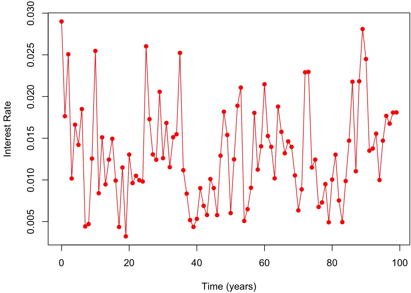
6.5.2.5 Inference for Multivariate SDE Models
Before making parameter inference, we give a brief description of the MCMC algorithm used by msde.
The MCMC initialization is conducted with the \(m\)-level Euler approximation as the following: suppose that the interobservation time is \(\Delta t\), then for any integer \(m > 0\), we define \(\boldsymbol{Y}_{(m)} = (\boldsymbol{Y}_{m, 0}, \ldots, \boldsymbol{Y}_{m, Nm})\) to be the value of SDE at equally spaced intervals of \(\Delta t_m = \Delta t / m\). If \(m = 1\), then \(\boldsymbol{Y}_{(m)} = \boldsymbol{Y}_{(1)} = \boldsymbol{Y}_{\text{obs}}\), which is the observed data. Moreover, for \(m > 1\), we have \(\boldsymbol{Y}_{m, nm} = \boldsymbol{Y}_n\). Intuitively, there are \(m-1\) equally spaced missing data points between observations. We define the missing data as \(\boldsymbol{Y}_{\text{miss}}\), then \(\boldsymbol{Y}_{\text{miss}} = \boldsymbol{Y}_{(m)} \setminus \boldsymbol{Y}_{\text{obs}}\).
The specific MCMC algorithm for sampling from posterior is a Metropolis-within-Gibbs sampler for each missing data point and parameter. The draws of the former use the proposal distribution introduced by Eraker (2001) and then demonstrated in Fang, Lysy, and Don (2020). In general, suppose \(\boldsymbol{Y}_t = (\boldsymbol{X}_t, \boldsymbol{Z}_t)\), where \(\boldsymbol{X}_t\) are observed components of size \(p\) and \(\boldsymbol{Z}_t\) are latent components of size \(q\). We can obtain the posterior density \(p(\boldsymbol{\theta} \mid \boldsymbol{X}_{0:N})\) by sampling from \(p(\boldsymbol{Z}_{0:N}, \boldsymbol{\theta} \mid \boldsymbol{X}_{0:N})\). However, we alternatively use a Gibbs sampler that samples from \(p(\boldsymbol{Z}_{0:N} \mid \boldsymbol{\theta}, \boldsymbol{X}_{0:N})\) and \(p(\boldsymbol{\theta} \mid \boldsymbol{Y}_{0:N})\) by a Metropolis-Hastings (MH) method.
In order to sample from \(p(\boldsymbol{Z}_{0:N} \mid \boldsymbol{\theta}, \boldsymbol{X}_{0:N})\), we sequentially update each component \(p(\boldsymbol{Z}_t \mid \boldsymbol{Z}_{-t}, \boldsymbol{\theta}, \boldsymbol{X}_{0:N})\), where \(\boldsymbol{Z}_{-t} = \boldsymbol{Z}_{0:N} \setminus \{\boldsymbol{Z}_t\}\). In particular, for the case where \(1 \leq t < N\), we use an MH algorithm with proposal density \(q(\boldsymbol{Z}_t \mid \boldsymbol{X}_t, \boldsymbol{Y}_{t-1}, \boldsymbol{Y}_{t+1}, \boldsymbol{\theta})\) such that the approximation to \(p(\boldsymbol{Y}_t \mid \boldsymbol{Y}_{t-1}, \boldsymbol{Y}_{t+1}, \boldsymbol{\theta})\) is:
\[
\boldsymbol{Y}_t \mid \boldsymbol{Y}_{t-1}, \boldsymbol{Y}_{t+1}, \boldsymbol{\theta} \sim \mathcal{N}_{p+q} \bigg(\frac{1}{2}(\boldsymbol{Y}_{t-1} + \boldsymbol{Y}_{t+1})), \frac{1}{2}\boldsymbol{\Sigma}_{t-1} \Delta t \bigg)
\]
where \(\boldsymbol{\Sigma}\) is the diffusion function.
After that, in order to draw from
\[
p(\boldsymbol{\theta} \mid \boldsymbol{Z}_{0:N}, \boldsymbol{X}_{0:N}) \propto \boldsymbol{\pi}(\boldsymbol{\theta}, \boldsymbol{Z}_0) \prod_{t=1}^N p(\boldsymbol{Y}_t \mid \boldsymbol{Y}_{t-1}, \boldsymbol{\theta}),
\]
we use vanilla random walk (with adaptive tuning) to update each component of \(\boldsymbol{\theta}\).
While using msde for parameter inference, the posteior sampling is achieved by the funcItôn sde.post. For the CIR model, we assume that there is no missing data, namely, m = 1. Note that missing data specification with function sde.init can be found here. Moreover, we use a Lebesgue prior \(\pi(\boldsymbol{\theta}) \propto 1\). Note that msde also allows default and custom prior specifications. Also note that we set the number of MCMC iterations, n_samples, to be 10000. The setting of this number is rather subjective and should be adjusted with respect to different SDE models.
# initialize the posterior sampler
init <- sde.init(model = cirmod, x = Xobs, dt = dT,
                 m = 1, theta = c(.1, .1, .1))

n_samples <- 1e5
burn <- 2e3
cirpost <- sde.post(model = cirmod, init = init,
                   hyper = NULL, #prior specification (Lebesgue prior)
                   nsamples = n_samples, burn = burn)
## Output size:## params = 60000## Running posterior sampler...## Execution time: 0.11 seconds.## gamma accept: 43.8%## mu accept: 43.3%## sigma accept: 43.9%# posterior histograms
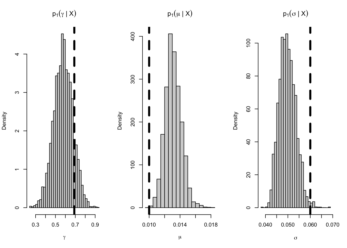
tnames <- expression(gamma, mu, sigma)
par(mfrow = c(1,3))
for(ii in 1:cirmod$nparams) {
hist(cirpost$params[,ii], breaks = 25, freq = FALSE,
xlab = tnames[ii],
main = parse(text = paste0("p[1](", tnames[ii], "*\" | \"*X)")))
# superimpose true parameter value
abline(v = theta0[ii], lwd = 4, lty = 2)
}
6.5.2.6 Summary
As can be seen from the posterior histogram above, it is convincing that Euler approximation does give an appropriate approximation to the true posterior density. Moreover, the above example gives a detailed tutorial on how to use msde for Bayesian parameter inference of SDE models. Readers are highly encouraged to run the above R and C++ codes on their own computers and use the tutorial as a template to make parameter inference for other SDE models.
Note that it is also possible to build the SDE model using TMB which allows users to implement C++ code in an R environment. The advantage of TMB is that, since the program is written in C++ and then compiled in R, it is more computer-efficient and thus takes much less time to run.
6.6 Appendix
6.6.1 Informal Proof for Itô’s Lemma
To get an insight into why the Itô’s lemma works, consider the argument below (what is shown below is not a formal proof of the Itô’s Lemma, but it gives an intuition on why the formula is right):
By the \(2^{nd}\) order Taylor expension:
\[\begin{align} X_{t} &\approx X_{0}+\frac{1}{1!}\Big(\frac{\ud X}{\ud t} \Big|_{t=0}\Big)(t-0)+\frac{1}{2!}\Big(\frac{\ud^2X}{\ud t^2} \Big|_{t=0}\Big)(t-0)^2 \\[3.5ex] \implies \ud X_t &\approx \frac{1}{1!}\Big(\frac{\ud X_s}{\ud s} \Big |_{s=t}\Big) \ \ud t + \frac{1}{2!} \Big(\frac{\ud^2 X_s}{\ud s^2} \Big |_{s=t} \Big) (\ud t)^2 \\[3.5ex] &= \Big(\frac{\ud (g(B_s))}{\ud s} \Big |_{s=t}\Big) \ \ud t +\frac{1}{2!}\Big(\frac{\ud^2 (g(B_s))}{\ud s^2} \Big |_{s=t} \Big)(\ud t)^2 && [X_s=g(B_s)]\\[3.5ex] &= \Big(\frac{\ud (g(g^{-1}(X_s))}{\ud s} \Big |_{s=t}\Big) \ \ud t + \frac{1}{2!} \Big(\frac{\ud^2 (g((g^{-1}(X_s))}{\ud s^2} \Big |_{s=t} \Big)(\ud t)^2 && [B_s=g^{-1}(X_s)]\\[3.5ex] &= \Big( g'(g^{-1}(X_s))\Big(\frac{\ud g^{-1}(X_s)}{\ud s} \Big) \Big |_{s=t} \Big\} \ud t +\frac{1}{2!} \Big( \frac{\ud^2 (g((g^{-1}(X_s))}{\ud s^2} \Big |_{s=t} \Big)(\ud t)^2 &&[\text{ Chain Rule }]\\[3.5ex] &= \Big\{ g'(g^{-1}(X_s))\Big(\frac{\ud B_s}{\ud s} \Big) \Big |_{s=t} \Big\} ud t + \frac{1}{2!} \Big(\frac{\ud^2 (g((g^{-1}(X_s))}{\ud s^2} \Big |_{s=t} \Big)(\ud t)^2 &&[g^{-1}(X_s)=B_s]\\[3ex] &= g'(g^{-1}(X_t)) \ \ud B_t +\frac{1}{2!}\Big\{\frac{\ud \Big(g'(g^{-1}(X_s))\Big(\frac{\ud g^{-1}(X_s)}{\ud s}\Big)\Big)}{\ud s} \Big |_{s=t}\Big \}(\ud t)^2 &&[\text{ Chain Rule }] \\[3.5ex] &= g'(g^{-1}(X_t)) \ \ud B_t + \frac{1}{2!} \Big \{ \Big(g''(g^{-1}(X_s))\Big(\frac{\ud g^{-1}(X_s)}{\ud s}\Big)^2 + g'(g^{-1}(X_s))\Big(\frac{\ud^2 g^{-1}(X_s)}{\ud s^2}\Big)\Big) \Big |_{s=t}\Big \}(\ud t)^2 &&[\text{ Product Rule }] \\[3.5ex] &\approx g'(g^{-1}(X_t)) \ \ud B_t +\frac{1}{2!}\Big \{g''(g^{-1}(X_s))\times T \Big\}, \\[2.5ex] &\approx g'(g^{-1}(X_t)) \ \ud B_t +\frac{1}{2!}g''(g^{-1}(X_s)) \ \ud t \end{align}\]
where:
\[ T = \Big(\frac{\ud g^{-1}(X_s)}{\ud s}\Big)^2 +\frac{1}{g''(g^{-1}(X_s))}\times \Big\{g'(g^{-1}(X_s))\Big(\frac{\ud^2 g^{-1}(X_s)}{\ud s^2}\Big) \Big\} \\ \]
6.6.2 The Itô Integral
The first step of the construction involves defining the integral for step processes. A step process is any stochastic process that can be written as \(X_t = \sum_{i = 1}^n X_{t_i} \: I_{[t_i, t_{i - 1}]}\). where \(I_A(t) = 1\) if \(t \in A\) and 0 otherwise. This is to say that \(X_t\) is a step process if we can find a partition such that the stochastic process is constant on each intervals. We will use the superscript \(X_t^n\) to indicate that there are \(n\) such intervals. We may then define the Itô integral of a step function \(X_t^n\) as follows: \[ I(X^n_t) = \int_a^b X^n_t \: \ud B_t = \sum_{i = 1}^n X_{t_i}(B_{t_i} - B_{t_{i-1}}) \] Here, we do not have to worry about the infinite variation since the integral is simply defined as a finite sum of random variables. We will try to use this as the springboard to extend the definition to non-step processes. To do this we first use the fact that, if \(X_{t}\) is a process where \(\int_a^b X_t^2 \: dt < \infty\), then there exists a sequence of approximating step processes such that: \[ \lim_{n \rightarrow \infty} E\bigg( \int_a^b (X_t^n - X_t)^2 \: \ud t \bigg) = 0 \qquad (*) \]
Our strategy will then be to use the the above convergence along with the fact that the integral \(I(X_t^n)\) is well defined to extend the integral to \(X_t\). We would hope that we can establish the result that no matter which approximating sequence \(X^n_t\) we choose, as long as \((*)\) holds then there exists an almost surely unique stochastic process \(Z_t\) such that:
\[ \lim_{n \rightarrow \infty} E\bigg(\big(Z_t - I(X_t^n)\big)^2 \bigg) = 0 \] Note that we are using the squared difference, and that this is inspired by our earlier discussion of the finite quadratic variation of brownian motion. It turns out that, provided \(X_t\) belongs to a certain class of well behaved stochastic processes (it is impossible to give further detail without delving into measure theoretic probability), that the above statement is true. We define the Itô the integral by setting \(I(X_t) = Z_t\).
We are now ready to define an SDE. It is simply any equation given in the following form:
\[ X_t = X_{t_0} + \int_{t_0}^t \mu(s, X_s) \: \ud s+ \int_{t_0}^t \sigma(s, X_s) \ud B_s \] Notice that we added a term \(\sigma(s, X_s)\). This is because we may want to model our white noise as dependent on time or the value of the stochastic process \(X_t\). To abbreviate the above equation we write: \[ \ud X_t = \mu(s, X_t) \ud t + \sigma(s, X_s) \ud B_s \] However, it should be kept in mind that this is only a short form for the integral equation given above. Any random variable \(X_t\) which satisfies the integral equations, is a solution to the SDE.