Chapter 4 Gaussian Processes
This section introduces the basic idea of the Gaussian Process. In an informal sense, if we consider infinite number of univariate Gaussian distributions which are correlated and combine all of them together, essentially we will have a multivariate Gaussian. A Gaussian process can be considered as a collection of Gaussian random variables.
4.1 Kernel
At the core of Gaussian processes is the choice of kernel as it encodes the unique properties of a Gaussian process. Before we dive into the discussion of Gaussian processes, we will start by introducing what a kernel is.
4.1.1 What is a kernel?
A kernel is a function \(k(\xx, \xx')\) that maps the inputs \(\xx\) and \(\xx'\) into a new space \(\mathbb{R}\). The entries of the covariance matrix of a Gaussian process are defined by the kernel. Essentially, the kernel is the covariance function that encodes our prior belief about the target function such as its smoothness. If we are interested in the function value at a new point, a smooth function means its neighbouring points can provide a lot of information about its value. However, for a rough function, we cannot infer much information about it from its neighbours. Note that we are talking about the smoothness of the target function instead of the kernel. In conclusion, the intuition is that the kernel measures the correlation between two points and there should be higher correlation for points closer to each other.
4.1.2 How do I choose the kernel?
It depends on your modeling problem, as there is no one-size-fits-all kernel. However, there are requirements that a kernel must satisfy: it has to be symmetric and positive semidefinite so the resulting covariance matrix is well-defined.
It is common in practice to choose kernels that are stationary or isotropic. For two inputs \(\xx\) and \(\xx'\), a stationary kernel is a function of \(\xx-\xx'\), i.e. \(k(\xx, \xx')=g(\xx-\xx')\) for some function \(g(\cdot)\). Such kernels only depend on the direction and the length of the difference between two input values. Isotropic kernels are a special case of stationary kernels. Such kernels only depend on the norm of \(\xx-\xx'\), i.e. \(k(\xx, \xx')=g({\Vert \xx-\xx'\Vert})\). Some examples of isotropic kernels are given in the following.
Examples
Squared exponential covariance function: \[k(\xx, \xx') = \sigma^2 \exp\left(-\frac{\Vert\xx-\xx' \Vert^2}{2\lambda^2}\right), \] where \(\lambda\) is called the length-scale parameter. The length-scale parameter \(\lambda\) is the distance you have to move on the input space to observe a significant change in the output space, so it can be thought of as approximately the distance between two peaks (both higher and lower) on the output function. It has the nice property of being very smooth as it is infinitely differentiable.
Matérn function: \[k(\xx, \xx') = \frac{2^{1-\nu}}{\Gamma(\nu)}\Big(\frac{\sqrt{2\nu}\Vert\xx-\xx' \Vert}{\lambda}\Big)^{\nu}K_{\nu}\Big( \frac{\sqrt{2\nu}\Vert\xx-\xx' \Vert}{\lambda}\Big), \] where \(K_{\nu}\) is the modified Bessel function of the second kind and \(\nu\) determines how smooth the function is. As \(\nu \rightarrow 0\), the Matérn function reduces to the squared exponential covariance function. If \(\nu=0\), it becomes the Ornstein-Uhlenbeck process kernel, which results in very rough output function. In Figure 4.1 shows how the choice of \(\nu\) affect the smoothness of the function.
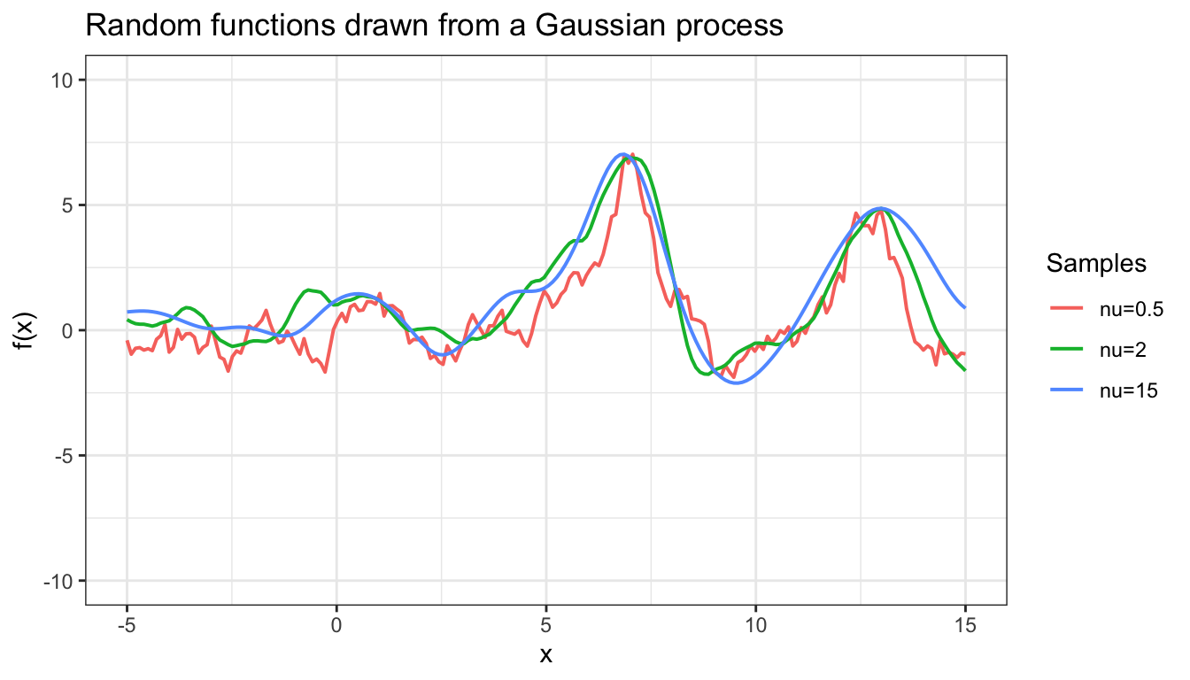
Figure 4.1: Samples from GP using kernels with different values of nu
If we choose a kernel that results in a very smooth function, it might be able to generalize more broadly beyond the training data, but is it able to capture complex dependency among the data? So how do we choose an appropriate smoothness? Suppose we want to use the Gaussian process to model eye movement and pedestrian trajectory, both of which can be summarized by a time-dependent function. While the direction of eye movement can change rapidly, resulting in a relatively rough function, pedestrain trajectory is more likely to be smooth. Therefore, it is more sensible to use a kernel that results in a smooth function for the Gaussian process model for pedestrain trajectory.
Some useful references on kernels are:
4.2 Gaussian Process Regression
In this subsection the training set \(\mathcal{D}\) of \(N\) observation is defined as: \[ \mathcal{D} = \{ (\xx_i,y_i)| i = 1,...,N\};\] where \(\xx_i\) is an input column vector with \(P\) features, and \(y_i\) is a scalar output (target). Based on this setup, the \(P \times N\) design matrix \(\XX\) is the collection of the \(N\) input column vectors, and the \(N \times 1\) target vector \(\yy\) is the collection of the \(N\) scalar outputs. Before moving on to the Gaussian process regression model, it makes more intuitive sense to review some of the concepts of Bayesian Linear Regression, and then connect the Bayesian Linear Regression model with Gaussian process regression.
4.2.1 Weight-Space View
For the Bayesian Linear Regression model, the prediction function is a linear combination of all the features, and all the \(p\) parameters (weights) can be estimated from the model, which is also referred as the parametric model. For Bayesian Linear Regression with Gaussian prior, the model can be expressed as: \[ y_i = \ww^T\xx_i + \epsilon_i, \]
where \(\ww^T = (w_1, w_2, ..., w_p)\) are the weights following a multivariate Gaussian distribution, and \(\epsilon_i \overset{iid}{\sim}\mathcal{N}(0,\sigma_\epsilon^2)\).
We assume the Gaussian prior has mean = \(\bm{0}\) and covariance = \(\bm{\Sigma}_P\), i.e. \(\ww\sim \mathcal{N}(\bm{0},\bm{\Sigma}_P)\), and the conditional distribution of the \(N\) observations can be written as: \[\begin{align*} p(\yy|\XX, \ww) &= \frac{1}{\sqrt{2\pi\sigma_\epsilon^2}}{\cdot} {\exp}\left[-\frac{1}{2\sigma_\epsilon^2}(\yy - \XX^T\ww)^T(\yy - \XX^T\ww)\right]\\ &\sim \mathcal{N}(\XX^T\ww, \sigma_\epsilon^2\bm{I}_{N{\times}N}). \end{align*}\]
And the prior can be written as: \[\begin{align*} p(\ww) &= \frac{1}{(2\pi)^{p/2}|\bm{\Sigma}_P|}{\cdot} {\exp}\left[-\frac{1}{2}\ww^T\bm{\Sigma}_P^{-1}\ww\right] \\ &\sim \mathcal{N}(\bm{0}, \bm{\Sigma}_P). \end{align*}\]
Since inference in the Bayesian Linear Regression model is based on the posterior distribution, it is crucial to find the posterior distribution using the Bayes’ rule and combine it with the assumptions above, i.e. \[ p(\ww|\yy,\XX) = \frac{p(\yy|\XX,\ww) p(\ww)}{p(\yy|\XX)},\]
where, \[ p(\yy|\XX) = {\int}p(\yy|\XX,\ww)p(\ww)d\ww.\]
The denominator in the posterior distribution is integrated over \(\ww\), and all the other variables are known in this integration. Therefore, this term can be treated as a normalizing constant, and can be ignored at the stage of determining the posterior distribution. By removing the normalizing constant from the Bayes’ equation, the posterior density function can be simplified to: \[\begin{align*} p(\ww|\yy,\XX) &\propto p(\yy|\XX,\ww) p(\ww) \\ &= {\exp}\left[-\frac{1}{2\sigma_\epsilon^2}(\yy - \XX^T\ww)^T(\yy - \XX^T\ww)\right] {\exp}(-\frac{1}{2}\ww^T\bm{\Sigma}_P^{-1}\ww) \\ &\propto {\exp}\left[-\frac{1}{2\sigma_\epsilon^2}(-2\ww^T\XX\yy + \ww^T\XX \XX^T\ww) - \frac{1}{2}\ww^T\bm{\Sigma}_P^{-1}\ww\right] \\ & \ \ \ \ \ \ {\times}\exp\left[-\frac{1}{4\sigma_\epsilon^4}\yy^T\XX^T (\sigma_\epsilon^{-2}\XX\XX^T + \bm{\Sigma}_P^{-1})\XX\yy\right] \\ &={\exp}\left[-\frac{1}{2}(\ww-\sigma_\epsilon^{-2}\bm{A}^{-1}\XX\yy)^T\bm{A} (\ww-\sigma_\epsilon^{-2}\bm{A}^{-1}\XX\yy)\right] \\ &\sim \mathcal{N}(\sigma_\epsilon^{-2}\bm{A}^{-1}\XX\yy,\bm{A}^{-1}), \end{align*}\]
where \(\bm{A} = \sigma_\epsilon^{-2}\XX\XX^T + \bm{\Sigma}_P^{-1}.\)
The above formulation returns the same distribution (with different parameter values) as that of the observations. In Bayesian statistics, the prior distribution in this formulation is also called a Conjugate Prior. It means that, by using the Conjugate Prior, the posterior distribution will be in the same distribution class as the prior.
On the other hand, the prediction on the test data can be achieved by weighted average of the density functions using the posterior distributions as the weights: \[\begin{align*} \text{i.e. } p(f_\ast|x_\ast,\XX,\yy) &= {\int}p(f_\ast|x_\ast,\ww) p(\ww|\yy,\XX)d\ww \\ &\sim \mathcal{N}(\sigma_\epsilon^{-2}x_\ast^T\bm{A}^{-1}\XX\yy, x_\ast^T\bm{A}^{-1}x_\ast). \end{align*}\]
4.2.2 Function-Space View
In the previous part on the weight-space view, there was a strong assumption made on the Linear Regression model that assumes a linear relationship between the features and the outputs. To address this issue, one can map the current features space into a higher dimensional space by some predefined transformation functions; however, this will give rise to another problem, which is there are infinitely many potential candidates for the transformation function. Therefore, the function-space view can be used to address this issue. In function-space view, there is no explicit form for the transformation functions, and it uses a kernel function to map the features into a high dimension space, which can be used to approximate different shapes of curves.
Gaussian process regression adopts this function-space view, and applies a Gaussian Process on the functional values, which can be thought as a multivariate Gaussian distribution over the function. And formally:
Definition: A Gaussian process is a collection of random variables, any finite number of which have a joint Gaussian distribution. (Rasmussen and Williams 2006)
A Gaussian process over a prediction function \(f(x)\) can be completely specified by its mean function and covariance function (or kernel function), \[ \text{Gaussian process: } f(\xx) \sim \mathcal{GP}(m(\xx),k(\xx,\xx')),\] where \[\begin{align*} \tx{mean function: } \ m({\xx}) &= E[f({\xx})],\\ \tx{covariance function: } \ k({\xx},{\xx}') &= E[(f({\xx})-m({\xx}))(f({\xx}') - m({\xx}'))]. \end{align*}\]
Therefore, the Gaussian process is an non-parametric approach, where the functions of these features are unspecified, and it is expressed by a Gaussian process with the predefined mean function as well as the kernel function.
For the Gaussian process discussed in this subsection, the two following assumptions are going to be assumed as default:
- The mean function \(m(\xx)\) is assumed to be 0.
- The squared exponential covariance function is used as the kernel, i.e. \[ k(\xx,\xx') = {\sigma^2}{\exp}\left[-\frac{1}{2\lambda^2}(\xx-\xx')^T(\xx-\xx')\right],\] where \(\lambda\) and \(\sigma\) are the two parameters in the kernel function controlling the horizontal scale and the vertical scale of the fitted curve, respectively.
The target \(\yy\) can be written as a combination of the Gaussian process function and a noise term, and in some cases, where the observations are assumed to be noise-free, the noise term can be removed from the model. The general formulation of the model is written as: \[\yy = f(\xx) + \bm{\epsilon}.\]
In addition to the \(P{\times}N\) design matrix \(\XX\), the testing data are defined as \(\XX_{P{\times}N_\ast}\), and the predicted test functional values are defined as \(\bm{f}_\ast\). By combining the testing data and training data, the prediction can be made using the joint Normal distribution, i.e. \[\begin{align*} \binom{\yy}{\bm{f}_\ast} \sim \mathcal{N}(\binom{\bm{0}}{\bm{0}}, \left( \begin{matrix} \bm{K} + {\sigma_\epsilon}^2\bm{I} & \bm{K}_\ast\\ \bm{K}_\ast^T & \bm{K}_{\ast\ast}\\ \end{matrix} \right)) \end{align*}\]
In this joint Normal distribution, the covariance matrix is in dimension \((N+N_\ast){\times}(N+N_\ast)\), and the input \(\bm{K}\) is \(N{\times}N\), \(\bm{K}_\ast\) is \(N{\times}N_\ast\), and \(\bm{K}_{\ast\ast}\) is \(N_\ast{\times}N_\ast\). Given the mean function and covariance function of the joint Normal distribution, it can be shown that the conditional expectation of the test functions also follows a normal distribution with mean \(\bm{\mu}_\ast\) and covariance \(\bm{\Sigma}_\ast\). Hence, the posterior distribution of the predicted functions for the test data is \[\begin{equation} \begin{split} p(\bm{f}_\ast|\XX_\ast,\XX,\yy) &\sim \mathcal{N}(\bm{f}_\ast|\mu_\ast,\Sigma_\ast), \\ \bm{\mu}_\ast &= \bm{K}_\ast^T(\bm{K} + {\sigma_{\epsilon}}^2\bm{I})^{-1}\yy, \\ \bm{\Sigma}_\ast &= \bm{K}_{\ast\ast} - \bm{K}_\ast^T(\bm{K} + {\sigma_{\epsilon}}^2\bm{I})^{-1}\bm{K}_\ast. \end{split} \tag{4.1} \end{equation}\]
4.2.3 Example - Gaussian Process Regression
Given the Gaussian process model defined in this subsection, the example in this part is going to use the Gaussian process regression to approximate a complicated function , which is defined as \[ f(x) = x\sin(x) - 0.1x^{\frac{1}{2}} + 0.5x^{\frac{1}{3}}\cos{(1.2x)}. \]
Figure 4.2 shows the values of the function \(f(x)\) at each input value of \(x\)
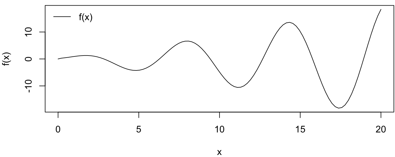
Figure 4.2: True Function
For the target variable \(y_i\), there is an extra layer of variation (\(\epsilon_i\)) added on top of the function \(f(x_i)\), and \(\epsilon_i\) is assumed to be i.i.d. \(\mathcal{N}(0,0.1^2)\) random variables. \[ y_i = f(x_i) + \epsilon_i, \] Therefore, in this simple example, the only part in the equation that needs to be predicted from the model is the unknown function, \(f(x)\), and a strong assumption has been made in this example that the value of \(\sigma_\epsilon\) is given to be 0.1; however, in a more realistic Bayesian model, this parameter, \(\sigma_\epsilon^2\), is usually unknown, and can be assumed as a random variable, which requires a hierarchical structure to model this randomness.
Given the model structure, 10 observations were sampled and then displayed in Table 4.1, which includes the target outputs, the functional values, and the sample points. On the other hand, the test data were 100 points sampled at equal step-size from 0 to 25. \[ \text{i.e. } \XX_{N_\ast} = (x_1, x_2, ..., x_{100}) = (0, (2 - 1)\frac{25}{(100-1)}, ..., 25). \]
| y | f | x |
|---|---|---|
| -4.20356 | -4.19729 | 5.00000 |
| 2.10106 | 2.09922 | 6.66667 |
| 6.24652 | 6.25488 | 8.33333 |
| -4.83147 | -4.84742 | 10.00000 |
| -9.31987 | -9.32317 | 11.66667 |
| 7.74390 | 7.75211 | 13.33333 |
| 10.18613 | 10.18126 | 15.00000 |
| -13.52046 | -13.52784 | 16.66667 |
| -10.79008 | -10.79584 | 18.33333 |
| 18.38434 | 18.38739 | 20.00000 |
The next step is to find the covariance matrix of the joint distribution of the complete dataset given that a proper kernel function has been selected, and the squared exponential covariance function (with length scale = 1 and width scale = 1) is adopted in this example. A more rigorous selection of kernel function should be down with cross validation based on a selected loss function. Since the posterior distribution also follows a normal distribution and the parameter values of the distribution can be estimated from the kernel matrix, the remaining part will use linear algebra knowledge to solve the system of linear equations. The most complicated part in Equation (4.1) is the matrix inversion \(w.r.t\) \((\bm{K} + \bm{I})\), and this can be done by using Cholesky factorization given the matrix \((\bm{K} + \bm{I})\) is positive definite.
Having all the information ready, Figure 4.3 shows the result from using the Gaussian process regression to fit the target function. The plot shows the values of the true function \(f(x)\) from \(x = 0\) to 25, and the fitted curve using the test data with two standard deviation confidence intervals are also displayed. Three Gaussian processes (labeled “re-sample1”-“re-sample3”) were sampled from the posterior distribution of the predicted function, which show the variability of the predictions. The points on the curve indicates the 10 training points, which indicate that, by only using 10 points from the actual function, this simple Gaussian process regression can provide a pretty good fit to the curve.
Moreover, there are many things that can be improved from this simple model. For example, the assumption of the fixed noise term \(\sigma_\epsilon^2\) can be modeled with other distributions, and the hyperparameters (length scale \(\sigma^2\), width scale \(\lambda\)) can be tuned using cross validation. All of these improvement can be explored by the interested readers.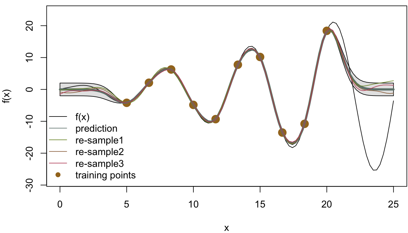
Figure 4.3: Gaussian process regression with C.I.
4.2.4 Practical Example - Kriging
In this example, we are going to use a practical example to illustrate how to estimate \(\sigma^2\) and \(\lambda\) in the kernel function. Kriging is a method of interpolation commonly used in geostatistics, which is essentially a Gaussian process regression. An example is the prediction of air pollutant concentration.
Suppose there are hundreds of air quality monitoring stations across Canada, and we are interested in predicting the air pollutant concentration in a town without a monitoring station. Let \(\XX\) denote the coordinates of different locations, and \(\yy\) denote the air pollutant concentrations at these locations. We can model the air pollutant concentration by \(\yy|\XX=\mu(\xx) + f(\XX)\), where \(\mu(\XX)\) is the trend of the concentration across locations. For the simplicity of this example, let’s assume the trend to be a constant vector of \(0\)s and the model is noise-free, i.e. \(\yy = f(\XX)\). Then we assume a Gaussian process model on \(f(\XX)\), which is given by \[ f(\XX) \sim \mathcal{N}(0, K(\XX, \XX)).\] where \(K(\XX, \XX)\) is defined by the exponential kernel \(k(\xx, \xx')=\sigma^2\exp(-\Vert\xx-\xx'\Vert/\lambda)\).
Let \(\xx_\ast\) be a new location where there is no monitoring station to provide an observation. We have \[\begin{bmatrix}f(\xx_\ast) \\ f(\XX)\end{bmatrix} \sim \mathcal{N}\left(\begin{bmatrix}0 \\ \bm{0} \end{bmatrix}, \begin{bmatrix} \sigma^2 & K(\xx_\ast, \XX)\\ K(\XX, \xx_\ast) & K(\XX, \XX). \end{bmatrix}\right)\] Since the conditional distribution of \(f(\xx_\ast)\big|f(\XX)\) is still Gaussian, \[ \begin{align*} f(\xx_\ast)\big|f(\XX) &\sim \mathcal{N}(m_{\tx{new}}(\xx_\ast), \sigma_{\tx{new}}(\xx_\ast)) \\ \tx{with } \ m_{\tx{new}}(\xx_\ast)&= K(\xx_\ast, \XX)K(\XX, \XX)^{-1}f(\XX),\\ \sigma_{\tx{new}}(\xx_\ast) &= \sigma^2 - K(\xx_\ast, \XX)K(\XX, \XX)^{-1}K(\XX, \xx_\ast). \end{align*} \]
Then the predicted mean value at location \(\xx_\ast\) is given by \(m_{\tx{new}}(\xx_\ast)\) with 95% confidence intervals \(m_{\tx{new}}(\xx_\ast)\pm 1.96\sigma_{\tx{new}}(\xx_\ast)\).
We will use simulation to demonstrate how kriging works in the following. In this example, we use the R package mvtnorm to simulate data from a multivariate normal distribution and optimCheck to check if likelihood optimization converges to a local mode. We also define a function solveV() that works faster on positive definite matrices than the R base function solve().
require(mvtnorm)
require(optimCheck)
source("code/solveV.R")
set.seed(946)
First, let’s simulate the data. The dataset is consisted of three variables: longitude, latitude, and air pollutant concentration.
# True parameters
sigma <- 2.4823
lambda <- 5.3342

# Simulate location coordinates
nsim <- 300
loc <- data.frame(lon = runif(nsim, 30,50), lat = runif(nsim, 10,70)) # longitude and latitude
dist <- as.matrix(dist(loc))
## Found more than one class "dist" in cache; using the first, from namespace 'spam'## Also defined by 'BiocGenerics'## Found more than one class "dist" in cache; using the first, from namespace 'spam'## Also defined by 'BiocGenerics'# Simulate air pollutant concentrations
cov_mat <- sigma * exp(-dist/lambda)
fx <- mvrnorm(1, rep(0, nsim), cov_mat)
data <- cbind(loc, fx)The dataset is divided into the observed (training) set and the new (test) set.
n_new <- floor(nsim*0.3) # We use 30% of the whole dataset as the test set
data_new <- data[1:n_new, ]
data_obs <- data[(n_new+1):nsim, ]
Define the negative log-likelihood function of the observed data to miminize over, which is essentially a multivariate normal distribution function.
nll <- function(par, data=data_obs){
  sigma <- par[1]
  lambda <- par[2]
  y <- as.vector(data[, 3])
  loc <- data[, c(1,2)]
  dist <- as.matrix(dist(loc))
  K <- sigma * exp(-dist/lambda)
  solve_output <- solveV(K, y, ldV = TRUE)
  logdet <- solve_output$ldV
  yK <- solve_output$y
  logdet + yK %*% y
}
Since we cannot obtain the estimates of \(\sigma^2\) and \(\lambda\) analytically, we will use the built-in optimization R function optim() to find the estimates numerically.
optim_result <- optim(c(3,10), nll)
sigma_hat <- optim_result$par[1]
lambda_hat <- optim_result$par[2]
optim_result
## $par
## [1] 3.926506 8.382991
##
## $value
## [1] 196.2254
##
## $counts
## function gradient
## 69 NA
##
## $convergence
## [1] 0
##
## $message
## NULLoptimCheck.
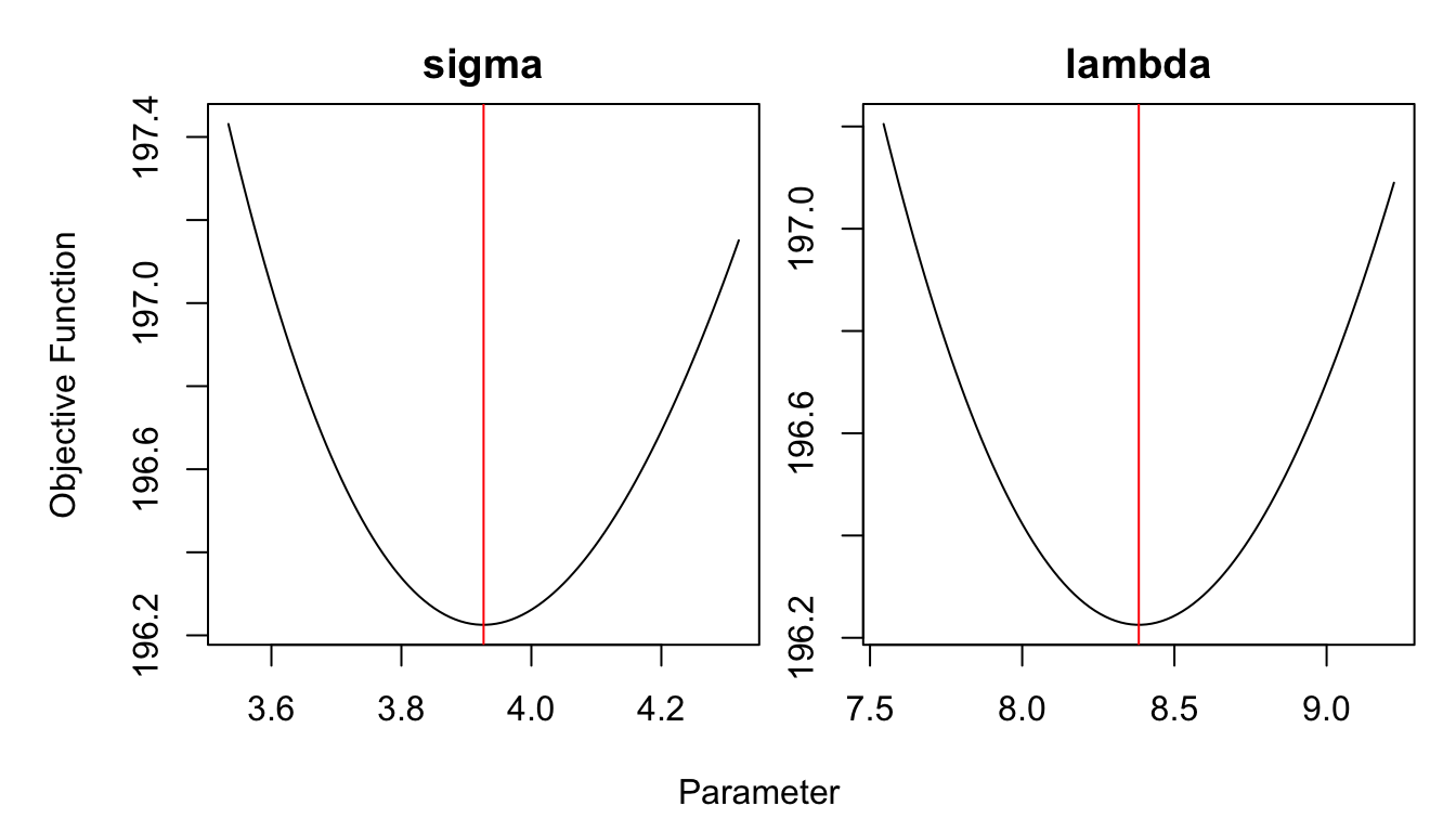
Figure 4.4: Hyperparameters optimization
After obtaining the parameter estimates, we can make predictions, and this step is called “kriging”. Given the observed data, the mean predicted values of the air pollutant concentration at the new locations can be computed using the formula of conditional mean of multivariate normal distribution.
# Obtain the distance matrix whose (i, j) entry is
# the distance between observation i and j in the dataset
dist_mat <- as.matrix(dist(data))
h_x_x <- dist_mat[(n_new+1):nsim, (n_new+1):nsim]
h_xs_x <- dist_mat[1:n_new, (n_new+1):nsim]

# Compute the covariance matrices of the underlying GPR.
k_x_x <- sigma_hat * exp(-h_x_x/lambda_hat) # The covariance among the observed data
k_xs_x <- sigma_hat * exp(-h_xs_x/lambda_hat) # The covariance between the observed data and the new data

# The conditional mean and covariance of the new data given the observed data
miu_star_hat <- k_xs_x %*% solve(k_x_x) %*% data_obs[, 3] 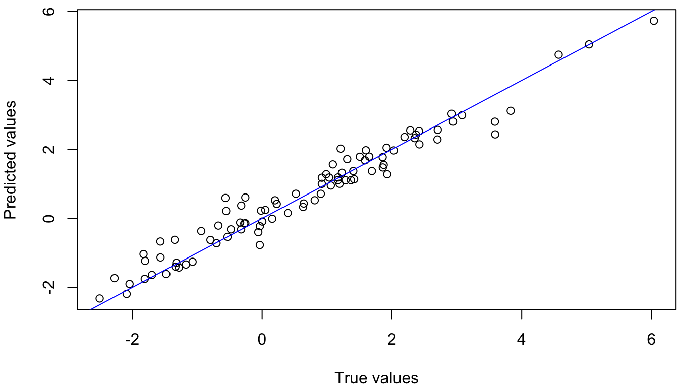
Figure 4.5: True VS Predicted Values
4.3 Classification
Now we introduce how the Gaussian process can be applied on classification of, in particular, binary data. Consider a simple binary classification problem where we observe an input \(\xx\) and the corresponding class label \(y \in \{-1, +1\}\). Given the observed data, we are interested in finding the class probability \(\pi(\xx_\ast)=p(y_\ast=+1|\xx_\ast)\) for a new input.
Using the logistic function \(\pi(\xx) = (1+e^{-f(\xx)})^{-1}\), we can put a Gaussian prior over \(f(\xx)\), which is a latent function as we are not directly interested in the form of \(f(\xx)\). Therefore, we have \[f(\xx)\sim \mathcal{N}(\xx'\bbe, K(\xx, \xx_\ast)).\]
In order to predict the class label of a new input \(\xx_\ast\), we will take the following steps:
Obtain the distribution of the latent variable \(f_\ast = f(\xx_\ast)\): \[p(f_\ast|\XX, \yy, \xx_\ast) = \int p(f_\ast|\XX,x_\ast,\bm{f})p(\bm{f}|\XX, \yy)d\bm{f}.\] where \(p(f_\ast|\XX,x_\ast,\bm{f})\) is Gaussian and \(p(\bm{f}|\XX, \yy)=p(\yy|\bm{f})p(\bm{f}|\XX)/p(\yy|\XX)\) is the posterior distribution of the latent variables.
Obtain the class probability: \[\pi(\xx_\ast) = p(y_\ast=+1|\XX, \yy, \xx_\ast) = \int p(y_\ast=+1|f_\ast) \ p(f_\ast|\XX, \yy, \xx_\ast)df_\ast,\]
Since both integrals are analytically intractable, we need to resort to Laplace approximation or methods based on MCMC sampling. In the following part, we will introduce how to approximate the posterior \(p(\bm{f}|\XX, \yy)\) using the Laplace approximation. For simplicity, let’s assume \(\bbe = \bm{0}\). We will use the model building functions from the TMB package in R to obtain parameter estimates. TMB combines automatic differentiation and Laplace approximation, and has the ability to handle hierarchical models with latent variables.
require(mvtnorm)
require(TMB)
require(ggplot2)
require(gridExtra)
library(RColorBrewer)
set.seed(946)
First, we will simulate the dataset, which contains \(N \times 2\) explanatory variables \(\XX\) and the binary class variables \(\yy \sim \tx{Bern}(\pi(\xx))\). For the kernel, we use an exponential covariance function.
nsim <- 500
# The true parameters
sigma <- 2.4823
lambda <- 5.3342

# Simulate the explanatory variables
x1 <- rnorm(nsim)
x2 <- rnorm(nsim)
X <- data.frame(x1=x1, x2=x2)
dist <- as.matrix(dist(X))

# Simulate the response variables
cov_mat <- sigma * exp(-dist/lambda)
fx <- rmvnorm(1, rep(0, nsim), cov_mat)
pi <- as.vector(1/(1+exp(-fx))) # class probabilities
# plot(density(pi))
class <- matrix(rbinom(nsim, 1, pi), nrow = nsim) # response variables
data <- cbind(X, class)
data$class <- as.factor(data$class)
data$class_probability <- pi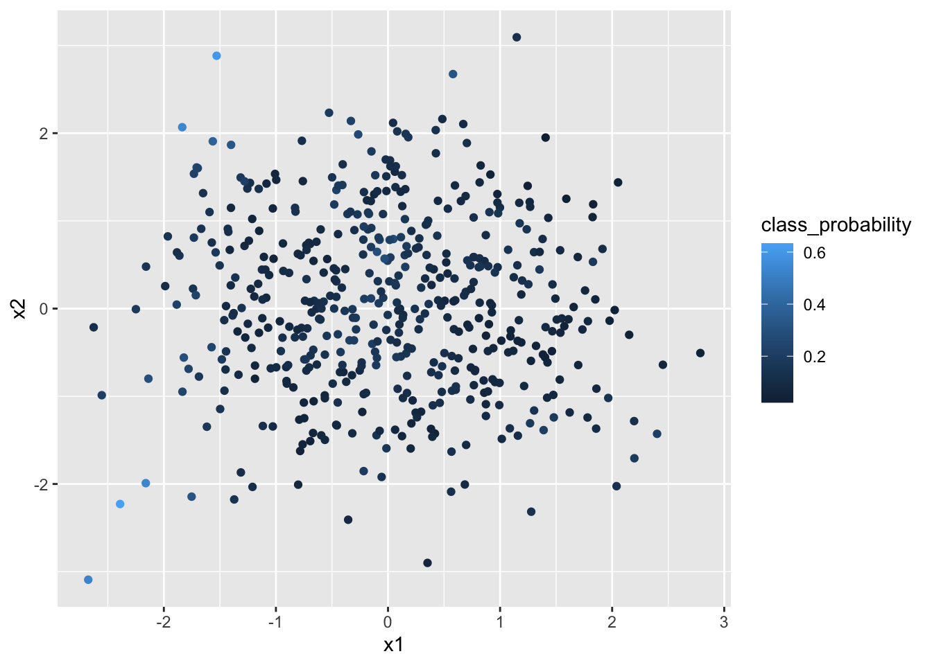
Figure 4.6: Class probabilites plotted on the input space
Now we divide the dataset into the observed set and the new set.
n_new <- floor(nsim*0.3)
data_new <- data[1:n_new, ]
data_obs <- data[(n_new+1):nsim, ]
The logistic-Gaussian model was written in a C++ file. We compile and load it into R using the compile() and dyn.load() functions in TMB package. The MakeADFun() function integrates out the latent variables \(\bm{f}\) and provides the negative log-likelihood function over which we will optimize to obtain the estimates of hyperparameters.
The function written in C++ takes in three data arguments: n: the number of observations, y: the binary response variables, and dd: the distance matrix whose \((i, j)\) entry is the Euclidean distance between \(\xx_i\) and \(\xx_j\).
Note that both hyperparameters \(\sigma^2\) and \(\lambda\) are transformed to log-scale so that the optimation is numerically stable. The initial values of \(\bm{f}\), \(\log(\sigma^2)\), and \(\log(\lambda)\) are set to be \((0, 0, \ldots, 0)^T\), \(0.5\), and \(1\), respectively.
compile("code/GPR_classification.cpp")
dyn.load(dynlib("code/GPR_classification"))
dd <- as.matrix(dist(data_obs[, c(1,2)]))
model <- MakeADFun(data = list(n=nrow(data_obs),
                               y=data_obs$class,
                               dd=dd),
                   parameters = list(f = rep(0, nrow(data_obs)),
                                     log_sigma = 0.5,
                                     log_lambda = 1),
                   random = "f",
                   DLL = "GPR_classification")
Then we use the built-in R optimization function to minimize the negative log-likelihood function provided by calling MakeADFun().
fit <- nlminb(model$par, model$fn, model$gr)fit## $par
## log_sigma log_lambda
## 1.698073 3.889491
##
## $objective
## [1] 116.1982
##
## $convergence
## [1] 0
##
## $iterations
## [1] 15
##
## $evaluations
## function gradient
## 16 15
##
## $message
## [1] "both X-convergence and relative convergence (5)"We can check, in Figure 4.7, that the optimization indeeded converged to local minima using the R package optimCheck.
require(optimCheck)
check_mode <- optim_proj(fun = model$fn, # objective function
           xsol = fit$par, # candidate optimum
           maximize = FALSE,
           xnames = c("sigma", "lambda"))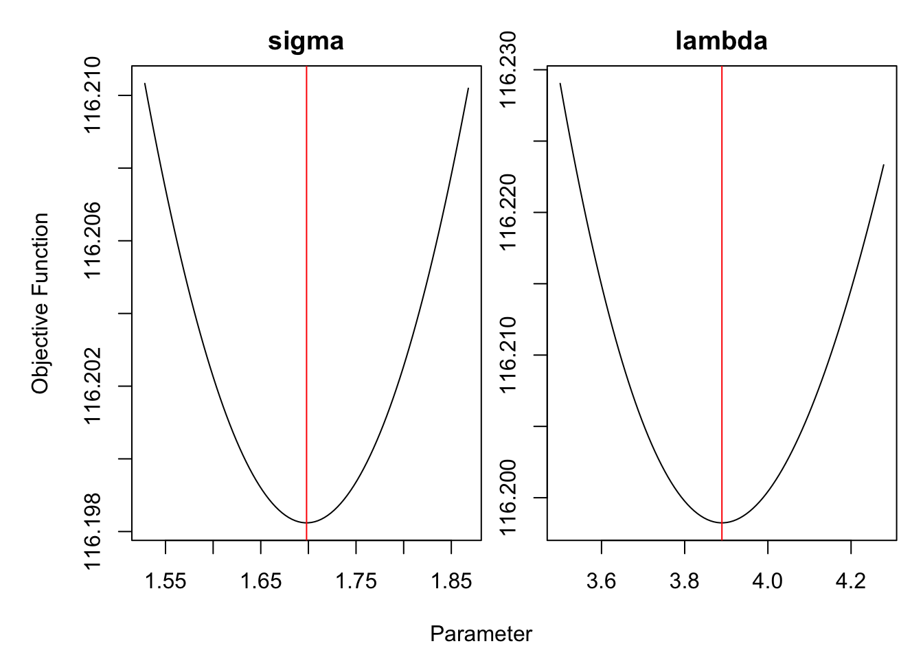
Figure 4.7: Hyperparameters optimization
Finally, we can make predictions using the estimated hyperparameters. Given the observed data, we use the formula of conditional mean of multivariate normal distribution to obtain the mean values of the latent functions \(\bm{f}_\ast\). Then the class probabilities are given by applying the logistic function on \(\bm{f}_\ast\).
In Figure 4.8, the predicted class probabilities are plotted against the simulated class probabilities. Data points belonging to class 1 are colored blue, and the ones in class 0 are colored red. It can be observed that the data roughly lie on a diagonal line, suggesting that the logistic-GP model does have prediction power. The data points on the right side of the plot are mostly blue, which corresponds to the fact that points with higher class probability are more likely to belong to class 1.
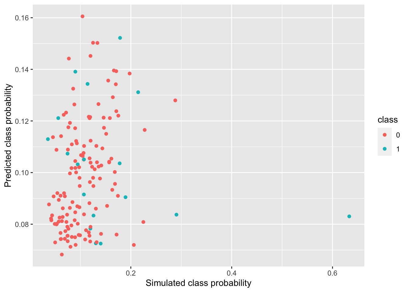
Figure 4.8: Predicted VS Simulated Class Probabilities
In Figure 4.9, both the predicted class probabilities and the true class labels are plotted on the input space, where the x-axis corresponds to the \(x_1\) variable and the y-axis corresponds to the \(x_2\) variable. When we compare the plot on the left with Figure 4.6, which plots the simulated class probabilities on the input space, we can observe similar patterns. Both plots have more points with lighter color on the left, which corresponds to higher probability of belonging to class 1. Therefore, the GP model component is able to capture the distribution of class probabilities.
We also compare the plot on the left to the one on the right, which shows how true class labels of the test data are distributed on the input space. It can be observed that more red points appear on the right side of the plot, which agrees with having more dark points on the right for the plot on the left.
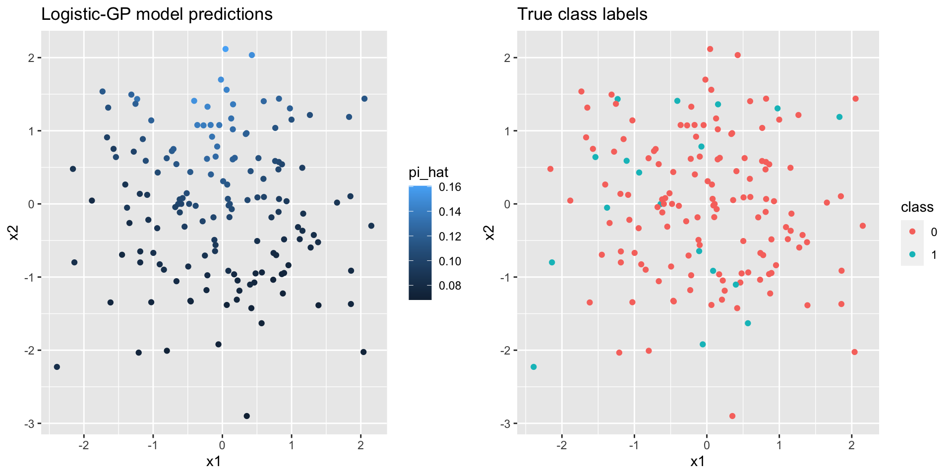
Figure 4.9: Predicted class probabilites and true class labels plotted on the input space
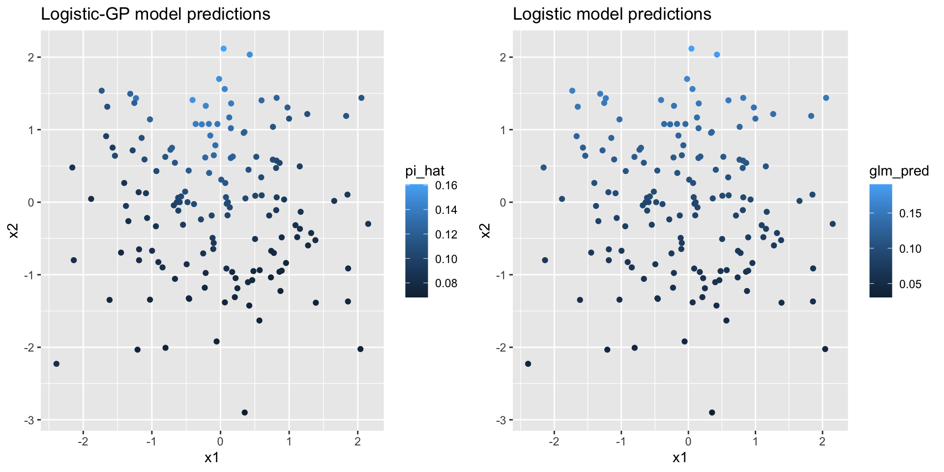
Figure 4.10: Predicted class probabilites and true class labels plotted on the input space
rbinom() function, we do not want to use a simple thresholding method like ifelse(pi_hat>0.5, 1, 0) to obtain the class label of a new data point. We generated binary data from Bernoulli distributions \(\tx{Bern}(\hat{\pi}(\xx_\ast))\), and compared them with the true class labels, with both plotted on the input space (Figure 4.11). Even though we only have a moderate size of data with 150 new observations, we still observe similar patterns of color distribution on the input space, which means we were able to recover the data generating process.
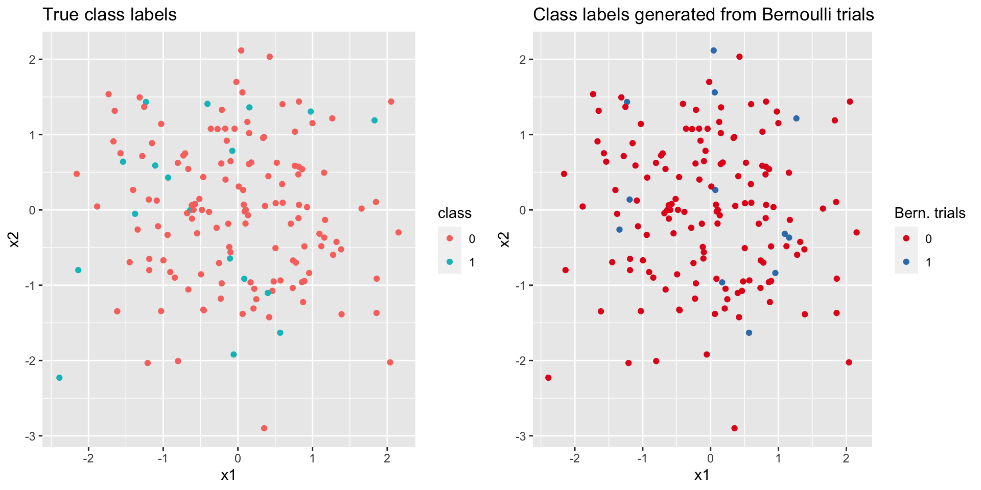
Figure 4.11: Comparison of true class labels and the class labels from Bernoulli trials
4.4 Computational Challenges
Though the Gaussian process offers a flexible modeling framework for us to specify the dependency among data, it suffers from computational complexities in the face of big data. The problem is rooted in the covariance matrix. One of the complexities is having a non-invertible covariance matrix, which is often called an ill-conditioned matrix. It occurs when we have two or more observations that are too close to each other on the input space. One remedy is by regularization, that is, adding a small constant (nugget) to the diagonal to make the matrix no longer singular. Readers interested in the regularization methods can refer to Radford M. Neal (1997) and Ranjan, Haynes, and Karsten (2011).
Gaussian processes are computationally expensive as they take into account the entire training data to make predictions, and inverting the covariance matrix is an operation of \(\mathcal{O}(n^3)\), where \(n\) is the size of training data. Common inference methods on the Gaussian process become numerically unstable when the size goes above a couple thousands. To approximate the process on a lower dimension, there is rich literature on sparse approximation of Gaussian processes, which incorporates a set of \(m\) latent variables \(\bm{u}=(u_1, \ldots, u_m)^T\) such that \(m < n\). The latent variables \(\bm{u}\) are commonly referred to as “inducing variables”, “active set”, or “pseudo-inputs” (Quinonero-Candela and Rasmussen 2005; Snelson and Ghahramani 2006). In the remainder of this subsection, we will introduce how sparse approximation is carried out for Gaussian processes.
4.4.1 Sparse Approximation of Gaussian processes
Consider a Gaussian regression model \[\begin{align*} y_i & = f(\xx_i) + \epsilon_i, \\ \tx{where } \ \epsilon &\sim \N(0, \sigma_\epsilon^2), \\ \bm{f}|\XX &\sim \N(\bm{0}, \bm{K}). \end{align*}\]
Alternatively, the model can also be written as \[ \yy|\bm{f} \sim \N(\bm{f}, \sigma_\epsilon^2\bm{I}) \]
Equation (4.1) gives the predictive distribution when we use the full covariance matrix, which is obtained by the following marginalization \[ p(\bm{f}_\ast|\XX_\ast, \XX, \yy) = \frac{1}{p(\yy)}\int p(\yy|\bm{f})p(\bm{f}, \bm{f}_\ast)d\bm{f}.\]
We can reduce the computational complexity by approximating the prior \(p(\bm{f}, \bm{f}_\ast)\), which is achieved by introducing the set of inducing variables \(\bm{u}=(u_1, \ldots, u_m)^T\) with \(m < n\), such that \[ \bm{u} \sim \N(\bm{0}, \bm{K_{u,u}}) \]
We approximate the prior by assuming that \(\bm{f}_\ast\) and \(\bm{f}\) are conditionally independent given \(\bm{u}\), i.e. \[\begin{equation} p(\bm{f}_\ast, \bm{f}) \approx q(\bm{f}_\ast, \bm{f}) = \int q(\bm{f}_\ast|\bm{u})q(\bm{f}|\bm{u})p(\bm{u})d\bm{u}, \tag{4.2} \end{equation}\] Where \(q(\cdot)\) is the approximate distribution. This is the fundamental of sparse approximation of Gaussian process, which using the inducing variable to build a conditional independent structures between the training data and the testing data, hence greatly reduced the computation costs. Before we introducing different conditional independent structure, we would like to state the forms of exact conditional distributions (without the noise term) at below, \[\begin{equation} \begin{aligned} \tx{Observed data: } \ \ \ p(\bm{f}|\bm{u}) &= \N(\bm{K_{f,u}}\bm{K_{u,u}}^{-1} \ \bm{u}, \bm{K_{f,f}}-\bm{Q_{f,f}}) \\ \tx{New data: } \ \ \ p(\bm{f}_\ast|\bm{u}) &= \N(\bm{K}_{\ast,\bm{u}}\bm{K_{u,u}}^{-1} \ \bm{u},\bm{K}_{\ast,\ast}-\bm{Q}_{\ast,\ast}), \end{aligned} \tag{4.3} \end{equation}\] where \(\bm{Q_{a,b}} \overset{\Delta}{=}\bm{K_{a,u}}\bm{K_{u,u}}^{-1}\bm{K_{u,b}}\).
In this part, we would like to introduce two conditional independent structures,
Subset of Regressors (SoR)
Fully Independent Training Conditional (FITC)
The first model is mathematically friendly but not very useful in practice, and the second model is more practical but have a more complicated form. Therefore, we will begin with deriving the equations for the the first model, and the result of the second model should come out naturally.
For the SoR, which are “finite linear-in-the-parameters models with a particular prior on the weights”(Silverman 1985; Smola and Bartlett 2001; Quinonero-Candela and Rasmussen 2005), the model structure we use to predict \(\bm{f}_\ast\) is then given by \[ \bm{f}_\ast = \bm{K}_{\ast, \bm{u}}\bm{w}_\bm{u}; \ \ p(\bm{w}_\bm{u}) \sim \N(\bm{0}, \bm{K}_{\bm{u}, \bm{u}}^{-1}), \] and it can be shown that, \[ \bm{f}_\ast= \bm{K}_{\ast, \bm{u}} \bm{K_{u,u}}^{-1} \bm{u}, \ \ \ \tx{with } \ \bm{u}\sim \N(\bm{0}, \bm{K_{u,u}}). \]
In this model, we assume there is a deterministic relation between \(\bm{f}_\ast\) and \(\bm{u}\), so the approximate conditional distributions in Equation (4.3) can be written as \[\begin{equation} \begin{split} \tx{Observed data: } \ \ \ q_{SoR}(\bm{f}|\bm{u}) &= \N(\bm{K_{f,u}}\bm{K_{u,u}}^{-1} \ \bm{u}, \bm{0}) \\ \tx{New data: } \ \ \ q_{SoR}(\bm{f}_\ast|\bm{u}) &= \N(\bm{K}_{\ast,\bm{u}}\bm{K_{u,u}}^{-1} \ \bm{u},\bm{0}). \end{split} \tag{4.4} \end{equation}\]
Using Equation (4.2), the SoR model approximate prior is given by: \[\begin{align*} q_{SoR}(\bm{f}_\ast, \bm{f}) &= \int q_{SoR}(\bm{f}_\ast|\bm{u})q_{SoR}(\bm{f}|\bm{u})p(\bm{u})d\bm{u}\\ &= \N\left(\bm{0}, \begin{bmatrix} \bm{Q}_{\ast, \ast} & \bm{Q}_{\ast, \bm{f}} \\ \bm{Q}_{\bm{f},\ast} & \bm{Q_{f,f}} \end{bmatrix} \right), \end{align*}\] whose Normal form can be easily obtained as all components in the integral follow a Normal distribution. The block matrices of the covariance matrix is obtained by \[ \bm{K_{a,u}}\bm{K_{u,u}}^{-1} \ \cov(\bm{u, u}) \ \bm{K_{u,u}}^{-1} \bm{K_{u,b}} = \bm{K_{a,u}}\bm{K_{u,u}}^{-1}\bm{K_{u,b}}. \] Also recall that \(\bm{Q_{a,b}} \overset{\Delta}{=}\bm{K_{a,u}}\bm{K_{u,u}}^{-1}\bm{K_{u,b}}\).
Therefore, under the SoR model, we have \[ q_{SoR}(\bm{f}_\ast, \bm{y}) = \N\left(\bm{0}, \begin{bmatrix} \bm{Q}_{\ast, \ast} & \bm{Q}_{\ast, \bm{f}} \\ \bm{Q}_{\bm{f},\ast} & \bm{Q_{f,f}} + \sigma_\epsilon^2 \bm{I} \end{bmatrix} \right), \] and it follows that the predictive distribution is given by \[ q_{SoR}(\bm{f}_\ast|\bm{y}) = \N\big(\bm{Q}_{\ast, \bm{f}} (\bm{Q_{f,f}} +\sigma_n^2\bm{I})^{-1} \bm{y}, \ \bm{Q}_{\ast,\ast} - \bm{Q}_{\ast,\bm{f}} (\bm{Q_{f,f}}+\sigma_n^2\bm{I})^{-1} \bm{Q}_{\bm{f},\ast} \big) \]
In summary, we replace the covariance matrices \(\bm{K}\) with \(\bm{Q}\) to achieve approximation as \(\bm{Q}\) has rank \(m\). We can also think of this approach as replacing the kernel \(k(\xx, \xx')\) with \(k_{SoR}(\xx,\xx') = k(\xx,\bm{u}) \bm{K_{u,u}}^{-1} k(\bm{u}, \xx')\). The computation efficiency will be greatly improved by this approximation; however, the SoR models will suffer from the nonsensical predictive uncertainties due to the deterministic relation in the condition distribution (Equation (4.4)).
The FITC model assumes a more realistic structure on the two conditional independent distributions, which does not use the deterministic relation in the conditional distribution, and all the training points are conditionally independent to the inducing variable. The FITC model with a single test point is given as \[\begin{equation} \begin{split} \tx{Observed data: } \ \ \ q_{FITC}(\bm{f}|\bm{u}) &= \prod_{i = 1}^{n} p(f_i|\bm{u}) = \N(\bm{K_{f,u}}\bm{K_{u,u}}^{-1} \ \bm{u}, diag\left[ \bm{K_{f,f}} - \bm{Q_{f,f}}\right]), \\ \tx{New data: } \ \ \ q_{FITC}(f_\ast|\bm{u}) &= p(f_\ast|\bm{u}). \end{split} \tag{4.5} \end{equation}\]
And the predictive distribution is \[ q_{FITC}(f_\ast|\bm{y}) = \N(\bm{Q}_{\ast, \bm{f}}(\bm{Q_{f, f} + \bm{\Lambda}})^{-1}\bm{y}, \bm{K}_{\ast, \ast} - \bm{Q}_{\ast, \bm{f}}(\bm{Q_{f, f} + \bm{\Lambda}})^{-1}\bm{Q}_{\bm{f}, \ast}), \] where \(\bm{\Lambda} = diag\left[ \bm{K_{f, f} - \bm{Q_{f, f}} + \sigma_\epsilon^2\bm{I}} \right]\), and the computational complexity is identical to the SoR model. The FITC model does provide useful information to the prediction uncertainty, but it also encourages underestimation of the noise variance (Bauer, Wilk, and Rasmussen 2016), and a comparable method that can be used is called Variational Free Energy (VFE) approximation, which will not be introduced here.
After introducing the two sparse Gaussian process models, we would like to conclude this part with two examples to compare the SoR model and the FITC model, and the target function is going to be identical to the example in Gaussian process regression. The gptk package in R is a useful tool kit for Gaussian processes, and we used this package to complete the following examples in which, instead of comparing the run times, we compared the fits obtained from the sparse approximation with that from the full Gaussian process.
The result from the full Gaussian process with 25 training points is shown in Figure 4.12, which shows a good fit to the true function. In Figure 4.13 and Figure 4.14, we compared the full Gaussian process with SoR and FITC respectively. In the SoR model, it is hard to see the confidence intervals of the prediction function, which is the issue of SoR we mentioned before. On the other hand, the FITC model does provide more informative predictions with the two standard deviation confidence intervals colored in grey.
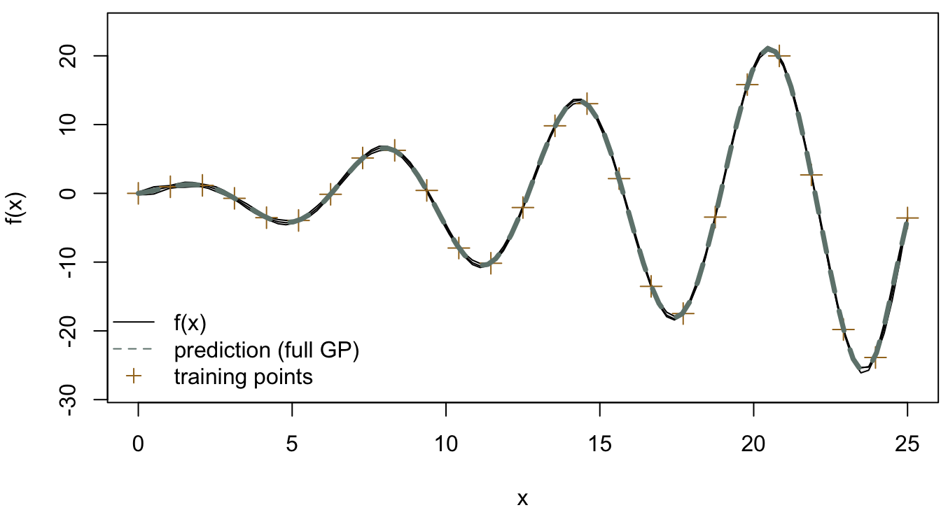
Figure 4.12: Full Gaussian process (25 training points)
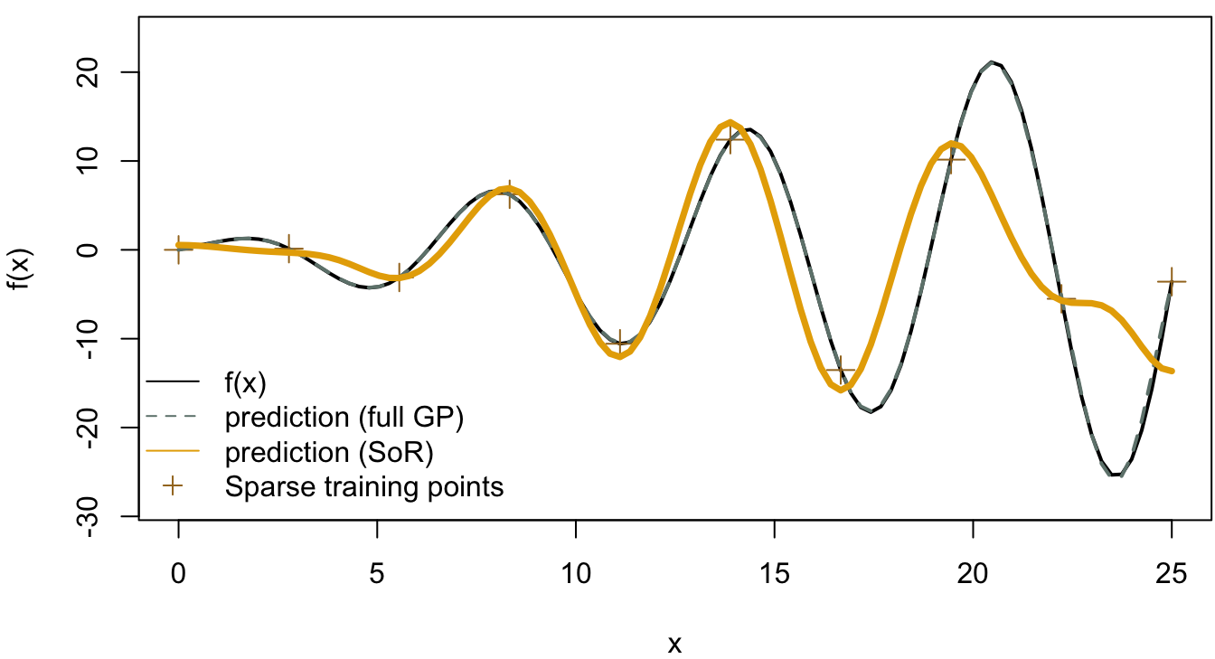
Figure 4.13: SoR model
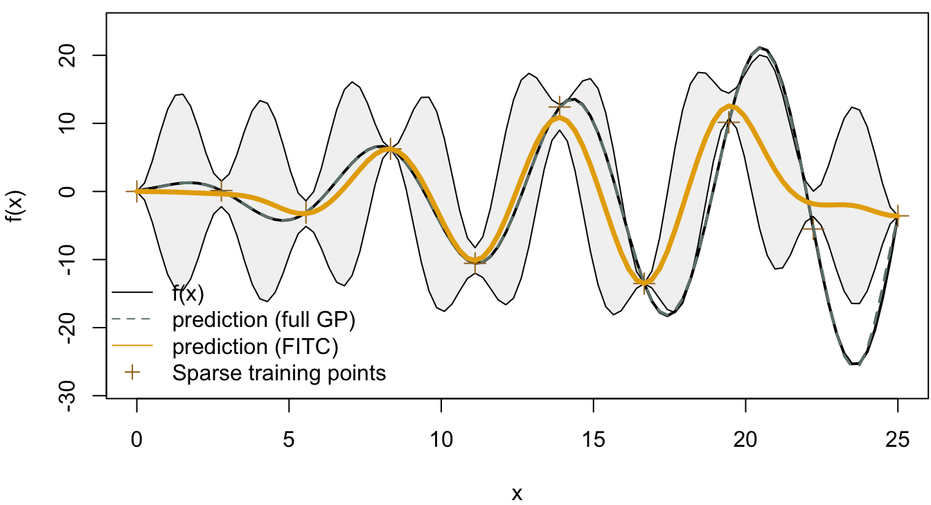
Figure 4.14: FITC model