Chapter 8 Laplace Approximation
8.1 Motivation
Suppose we have the following model set up, where \(\eet\) may be nuisance parameters or latent variables.
Model: \(\yy \sim p(\yy| \eet, \tth)\)
Prior: \(\eet \sim p(\eet \mid \tth)\)
Our main interest may be in finding estimates for the hyperparameters \(\tth\). We could use MCMC to explore the posterior distribution, but this is time-consuming, especially if our main interest is in \(\tth\) and we don’t care about accurately estimating \(\eet\). Instead, we can use the Laplace approximation to compute an approximation to the marginal likelihood \(\mathcal L(\tth \mid \yy)\) to find estimates for \(\tth\). The Laplace Approximation allows us to “integrate out” the nuisance parameters or latent variables, and deal directly with an approximation to the marginal likelihood.
8.2 Derivation
Before proceding, we will assume that the parameters in this model are all unconstrained. If any of the parameters are constrained, for example, \(\sigma > 0\), they should be transformed to an unconstrained scale before proceding, such as \(\lambda = \log(\sigma)\). The Laplace approximation always works better on the unconstrained scale.
We can write the likelihood of interest as:
\[\begin{align} \mathcal L (\tth \mid \yy) &\propto p(\yy\mid\tth) \\ &= \int p(\yy \mid \tth, \eet) p(\eet \mid \tth) \ud \eet \\ &= \int \exp (\ell(\tth \mid \yy, \eet)) \ud \eet \tag{8.1} \end{align}\]
Next, let \[ \hat \eet_{\tth} = \argmax_{\eet} \ell(\tth \mid \yy, \eet) \] denote the conditional maximizer of \(\ell(\tth \mid \yy, \eet)\) for fixed \(\tth\). We can expand \(\ell(\tth \mid \yy, \eet )\) using a quadratic Taylor approximation around its mode, \(\hat \eet_{\tth}\). Then we have: \[ \ell(\tth \mid \yy, \eet ) \approx \ell(\tth \mid \yy, \hat \eet_{\tth}) + \frac{1}{2} (\eet - \hat \eet_{\tth})' H_{\tth} (\eet - \hat \eet_{\tth}), \] where \(H_{\tth}\) is the Hessian matrix of \(\ell(\tth \mid \yy, \hat \eet_{\tth})\). Note that the first order term of the Taylor expansion is dropped, since \(\frac{\partial}{\partial \eet}\ell(\tth \mid \yy, \hat \eet_{\tth}) = 0\). Returning to Equation (8.1), we obtain:
\[ \begin{aligned} \mathcal L(\tth \mid \yy) &\approx \int \exp\left(\ell(\tth \mid \yy, \hat \eet_{\tth}) + \frac{1}{2} (\eet - \hat \eet_{\tth})' H_{\tth} (\eet - \hat \eet_{\tth})\right) d \eet \\ & \propto \exp\left(\ell(\tth \mid \yy, \hat \eet_{\tth}) - \frac{1}{2} \log \mid H_{\tth} \mid \right) \int \varphi(\eet \mid \hat \eet_{\tth}, H_{\tth}^{-1}) d\eet \end{aligned} \]
where \(\varphi(\eet \mid \hat \eet_{\tth}, H_{\tth}^{-1})\) is the PDF of a normal distribution and thus the integral is equal to one. Therefore, the Laplace approximation to \(\mathcal L(\tth \mid \yy)\) is given by \[ \mathcal L_{\tx{Lap}}(\tth \mid \yy) = \exp\left( \ell(\tth \mid \yy, \hat \eet_{\tth}) - \frac{1}{2} \log \mid H_{\tth} \mid\right), \]
or in other words, \[ \ellap(\tth \mid \yy)= \ell(\tth \mid \yy, \hat\eet_{\tth}) - \frac{1}{2} \log \mid H_{\tth} \mid \] Further, we can estimate the marginal posterior \(p(\tth \mid \yy)\) by a Normal distribution: \[ \tth \mid \yy \space \dot \sim \N(\hat \tth, \hat \SSi), \qquad \begin{array}{l} \hat \tth = \argmax_\tth \ellap(\tth \mid \yy) \\ \hat \SSi^{-1} = -\frac{\partial^2}{\partial\tth\partial\tth} \ellap(\hat\tth \mid \yy) \end{array} \]
The Laplace approximation works best when the marginal posterior distribution of \(\eet\) is symmetric and unimodal, since we are essentially approximating it using a Normal distribution. Further, Laplace works better when our sample size is large, due to asymptotic normality of the posterior distribution (Gelman et al. 2013). For a good explanation and justification for approximating marginal posterior distributions using the Normal, see Bayesian Data Analysis Chapter 4, Sections 4.1 and 4.2.
8.2.1 A Note on Terminology
Sometimes this method is referred to as the mode-quadrature approximation/procedure. The terms “Laplace approximation” and “mode-quadrature procedure” are ambiguous, and may refer to the entire procedure described in 8.2, or a subset of the steps. For example, approximating a distribution by a Normal with mean equal to the mode of the log likelihood and variance equal to the Hessian of the log likelihood evaluated at the mode may also be referred to as the mode-quadrature procedure (see Section??).
8.3 TMB for Laplace Approximations
The R package TMB is designed for fitting statistical latent variable and random effects models to data (a nice tutorial is available here). The user implements \(\ell(\YY, \tth, \eet)\) in , and TMB gives \(\ellap(\tth \mid \YY)\), and uses automatic differentiation to supply \(\frac{\partial}{\partial{\tth}} \ellap(\hat\tth \mid \YY)\) with no extra programming effort.
The user can then employ their desired optimization package to find \(\hat \tth = \argmax_{\tth} \ellap(\tth \mid \YY)\), and find \(\hat \SSi^{-1} = - \frac{\partial^2}{\partial \tth \partial\tth'} \ellap(\hat \tth \mid \YY)\) by numerically computing the derivative to \(\frac{\partial}{\partial{\tth}} \ellap(\hat\tth \mid \YY)\), which is supplied by TMB.
8.4 Example with TMB: Single Molecule FRET Microscopy
This is an example of a latent variable model where we will integrate out the latent variable via the Laplace approximation.
The distance between two molecules, \(X_t\), is a latent process which can be modeled as an Ornstein-Uhlenbeck process, that is \[ d X_t= -\gamma(X_t - \mu)\, \ud t + \sigma \, \ud B_t \] where \(\gamma >0,\, \sigma>0\), \(\mu\) is constant drift, and \(B_t\) refers to Brownian motion. This gives a continuous Gaussian Markov process with \[ \begin{aligned} X_0 & \sim \N(\mu, \tau^2) \\ X_{t+\Delta t} \mid X_t & \sim \N\left\{\mu + \rho_{\Delta t}\cdot(X_t - \mu), \tau^2 \cdot (1-\rho_{\Delta t}^2)\right\}, \end{aligned} \] where \(\tau^2 = \sigma^2/(2\gamma)\) and \(\rho_{\Delta t} = \exp(-\gamma \Delta t)\).
The observed data is \(\YY = (Y_1, ..., Y_N)\), the photon count measurements at times \(t_n = n\), where \[ Y_n \mid X_n \ind \exp(\beta_0 - \beta_1 X_n), \] where \(\beta_0\) and \(\beta_1\) are known experimental constants.
We will use TMB to find a Laplace approximation to \(\ell(\gamma, \sigma, \mu \mid \YY)\). Then we can use the stats::optim() function in R to find posterior estimates of the parameters of the Ornstein-Uhlenbeck process.
Note: We could also solve this problem via MCMC in Stan, however, the Laplace approximation is significantly faster.
To construct the TMB object which contains the negative log-posterior of \(\ell_{Lap}(\gamma, \sigma, \mu \mid \YY)\), you must supply the (negative) log likelihood for the complete data, which must be coded in C++. In this example, this code is in a file called smfret_ou.cpp. Here is a look at the main contents of this file:
#include <TMB.hpp>
template<class Type>
Type objective_function<Type>::operator() () {
  DATA_VECTOR(Y);
  DATA_SCALAR(dt);
  DATA_VECTOR(beta);
  PARAMETER_VECTOR(X);
  PARAMETER(log_gamma);
  PARAMETER(mu);
  PARAMETER(log_sigma);

  // intermediate variables
  Type lrho = -exp(log_gamma) * dt;
  Type rho = exp(lrho);
  Type tau = exp(log_sigma - Type(.5) * (log_gamma + log(Type(2.0))));
  Type nu = tau * sqrt(Type(1.0) - exp(Type(2.0) * lrho));
  vector<Type> lambda = exp(beta(0) - beta(1) * X);
  int N = Y.size();

  // output variable
  Type nll = Type(0.0);

  // latent variables
  nll += dnorm(X(0), mu, tau, 1); // initial value
  for(int ii=0; ii<N-1; ii++) {
    // subsequent values
    nll += dnorm(X(ii+1), rho * (X(ii) - mu) + mu, nu, 1);
  }
  // observed variables
  nll += sum(dpois(Y, lambda, 1));

  return -nll;
}
Notice that we log-transformed \(\sigma\) and \(\gamma\) to avoid dealing with their constraints. Let \(\pps = (\log(\gamma), \mu, \log(\sigma))\). Next, we simulate some data by picking some values for the parameters.
source("laplace/smfret-functions.R")
set.seed(500)
# simulate some data
beta0 <- 6
beta1 <- .5
gamma <- .2
mu <- 5.1
sigma <- .4
dt <- .1
n_obs <- 1000
X <- ou_sim(gamma = gamma, mu = mu, sigma = sigma, dt = dt, n_obs = n_obs)
Y <- rpois(n_obs, lambda = exp(beta0 - beta1 * X))
Now that we have data and we have coded the complete data negative log-likelihood, we can compile the model and create the \(\ellap(\pps \mid \yy)\) object using TMB::MakeADFun().
require(TMB)## Loading required package: TMB## Warning in checkMatrixPackageVersion(): Package version inconsistency detected.
## TMB was built with Matrix version 1.4.1
## Current Matrix version is 1.5.3
## Please re-install 'TMB' from source using install.packages('TMB', type = 'source') or ask CRAN for a binary version of 'TMB' matching CRAN's 'Matrix' package# compile the TMB code
mod_name <- "smfret_ou"
compile(paste0("laplace/",mod_name, ".cpp"))
dyn.load(dynlib(paste0("laplace/",mod_name)))
# Laplace approximate posterior
# for flat prior on psi = (log(gamma), mu, log(sigma))
# Construct the TMB object containing the
# negative log-posterior p_Lap(psi | Y)
# since E[Y | X] = exp(beta_0 - beta_1 * X),
# initialize with X = (beta_0 - log(Y+.1))/beta_1.
ou_adf <- MakeADFun(data = list(Y = Y, dt = dt,
beta = c(beta0, beta1)),
# parameter initialization
parameters = list(log_gamma = 0, mu = 0, log_sigma = 0,
X = (beta0 - log(Y+.1))/beta1),
# variables to approximately marginalize
random = "X",
silent = TRUE, DLL = mod_name,
checkParameterOrder = TRUE)Next, find the posterior mode using optim(), and check that we have indeed found the mode.
opt <- optim(par = c(0, 0, 0), # initial value
             fn = ou_adf$fn, # negative loglikelihood approximation
             gr = ou_adf$gr, # gradient of nll
             method = "BFGS") # gradient-base optimization

# check that we're indeed at the mode using optimCheck package
require(optimCheck)
## Loading required package: optimCheckoptim_proj(xsol = opt$par,
xnames = expression(log(gamma), mu, log(sigma)),
fun = ou_adf$fn, maximize = FALSE)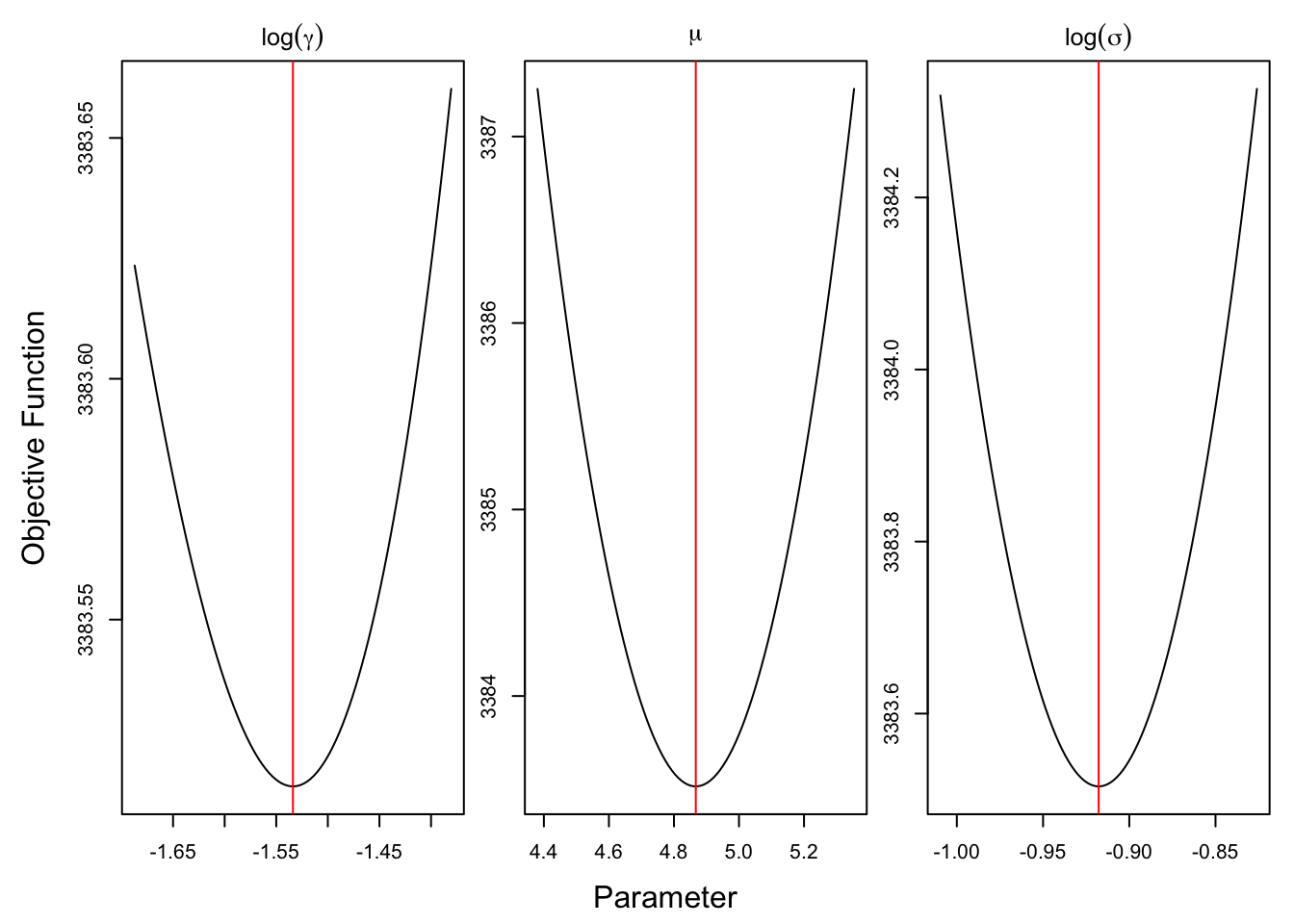
Now that we have found the posterior mode, we can use this as the mean of the normal approximation to the posterior distribution. In order to sample from our approximate posterior, we also require the variance, which we can get by numerically finding the Jacobian of the gradient supplied by TMB via autodiff. We can now sample from \(\hat p_{Lap}(\tth \mid Y)\) to get posterior samples. We must not forget to convert back to our original (constrained) parameter space.
# Use numDeriv package to get numerical Hessian from TMB
require(numDeriv)
## Loading required package: numDerivpsi_mean <- opt$par # posterior mode
# inverse posterior quadrature
# can't get TMB autodiff to compute gradient, so jacobian of gradient = hessian
psi_var <- numDeriv::jacobian(func = ou_adf$gr, x = opt$par)
psi_var <- chol2inv(chol(psi_var)) # fast + stable inversion of spd matrix
require(mniw) # fast calculations for multivariate normal## Loading required package: mniw# sample from p_Lap(psi | Y)
n_post <- 1e5
psi_post <- rmNorm(n_post, mu = psi_mean, Sigma = psi_var)
# convert to theta = (gamma, mu, sigma)
theta_post <- cbind(gamma = exp(psi_post[,1]),
mu = psi_post[,2],
sigma = exp(psi_post[,3]))Finally, we can plot the approximate posterior and compare it to the true parameter values (the black lines).
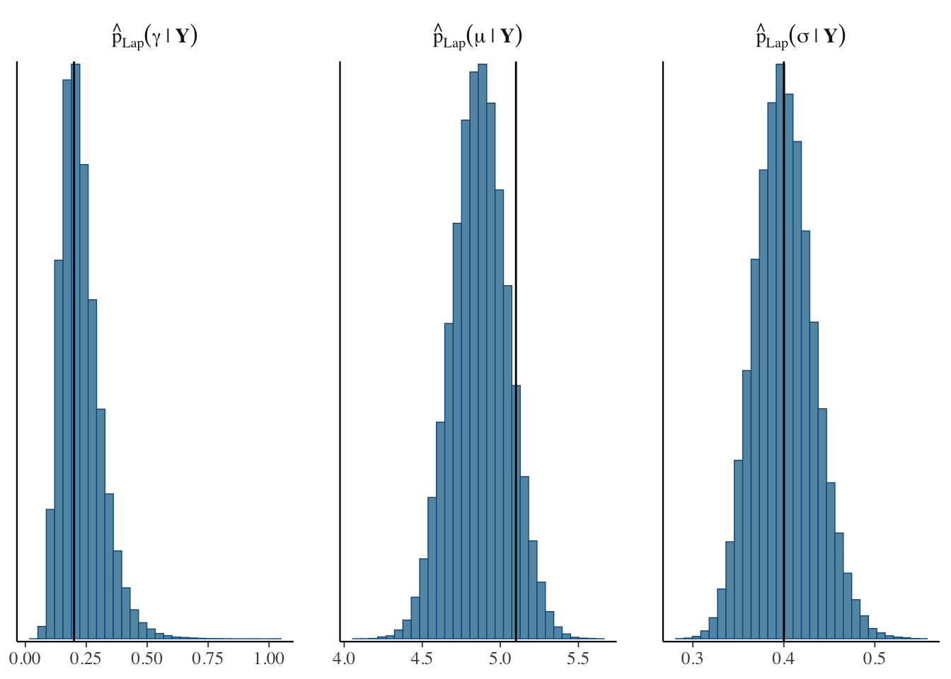
In this example, the Laplace approximation has given us pretty accurate estimates, particularly for \(\gamma\) and \(\sigma\), in significantly less time than exploring the whole posterior distribution using MCMC.
8.5 Applications
8.5.1 Estimating Uncertainty in Neural Networks
One nice aspect of the Laplace approximation is that it allows us to estimate the variance of the posterior distribution, offering a potential way to quantify the uncertainty of our estimates. This is particularly applicable to neural networks (NN), since these models are notoriously difficult to interpret and many lack a natural framework for uncertainty estimation.
A problem with the use of Laplace approximation for uncertainty estimation in NN is that it can require the Hessian matrix per each layer to be computed, which in most cases is computationally infeasible. This paper proposes a scalable approach to uncertainty estimation in neural networks using a Kronecker-factored (KFAC) Laplace approximation. In their experiments, the KFAC Laplace approximation performs slightly better than Dropout, which is another current method (Ritter, Botev, and Barber 2018).
This paper compares the relatively new and popular mean-field variational inference (MFVI) method to the linearised Laplace method for uncertainty estimation in NN. MFVI struggles to provide appropriately calibrated uncertainty estimates in regions between observed data (in-between uncertainty). Linearised Laplace (LL) outperforms MFVI for in-between uncertainty for smaller network architectures (Foong et al. 2019). However, MFVI is able to scale to much larger networks compared to LL. The authors suggest that future work should combine KFAC Laplace as proposed in (Ritter, Botev, and Barber 2018) with linearisation to obtain a more scalable and accurate solution to estimation of in-between uncertainty in Bayesian NN.
8.5.2 Integrated Nested Laplace Approximations and R-INLA package
Integrated Nested Laplace Approximation (INLA) is a combination of Laplace approximations and numerical integration techniques which can be applied to any model expressable as a latent Gaussian Markov random field (GMRF). This can encompass mixed-effect models, spatial and spatio-temporal models, survival analysis, and more. INLA can give very accurate estimates of posterior quantities while avoiding MCMC sampling, however, this method is only effective for models with a small number of parameters, less than about 15 (Martino and Riebler 2019).
Despite the restriction to GMRF models with relatively few parameters, INLA is worth mentioning because of the R-INLA package. It makes use of the INLA C library for fast approximate inference (the R package is actually just called INLA, but is referred to as R-INLA to distinguish between the two). R-INLA is extensively documented and widely used (see the R-INLA website, a GitHub book here, and a textbook with a focus on spatial modelling with stochastic partial differential equations here).