Chapter 5 Particle Filters
5.1 State-Space Models
5.1.1 Definition
A state-space model can be intuitively described as a latent time series paired with an observable, related time series. The former is referred to as the system model \(X_t\) and the latter as the measurement model \(Y_t\). The desired outcome is to be able to estimate the former using the latter.
More specifically, the evolution of the underlying system model from time \(t\) to \(t+1\) is a Markov chain. This means that the distribution of \(X_{t+1}\) is assumed to depend only on the previous system state \(X_t\); this is a relatively strong assumption, but also greatly simplifies the required work. The final piece of the state-space model is the measured value \(Y_t\); this quantity is only dependent on the unobserved system value \(X_t\) of the same time point.
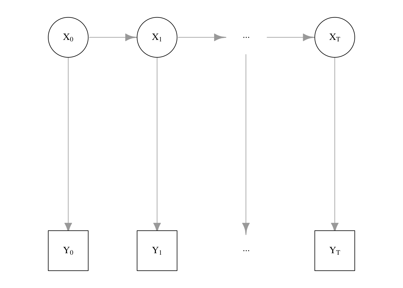
Figure 5.1: State-Space Model as a directed graph
The state-space model can also be depicted graphically as in Figure 5.1. An astute reader may notice that the graph structure strongly resembles that of a hidden Markov model; indeed, one may consider the state-space model as a generalization thereof. The primary difference is that the latent variable \(X_t\) is permitted to be a general (continuous) variable instead of a finite set of latent states. A particular choice of distribution on \(X_t\), such as the multinomial distribution, will allow us to recover hidden Markov models from state-space models.
The joint distribution of the complete model can be given in terms of the initial distribution \(\pi\), the conditional distribution of the Markov chain (state transition equation) \(f(X_t\mid X_{t-1})\), and the conditional distribution of the measured variable (observation equation) \(g(Y_t\mid X_t)\).
\[ p(\XX, \YY) = \pi(X_0) \times \prod_{t=1}^T f(X_t\mid X_{t-1}) \times \prod_{t=1}^T g(Y_t\mid X_t) \] We wish to estimate the unknown system values \(\XX\), ideally by obtaining \(p(\XX \mid \YY)\) or, as is much more likely in practice, sampling therefrom.
5.1.2 Illustrative Example
A common illustrative example of state is given in the context of robotics. Suppose we have a robot capable of moving about in a maze and that we have a complete map of the maze, but we don’t have a fix on the location of the robot. However, the robot is able to emit radar and measure the time it takes for the radar bounce to return from many directions in a 360-degree sweep. This distance indicates the proximity of a robot to a wall in that direction, and can be contaminated by spurious radar noise such as interference.
In this example, the underlying system model that we wish to estimate is the true position of the robot in the maze and the observable measureable model are the distances in various directions. As the robot moves, the true position changes and so, correspondingly, do the distance measurements.
Other real-world examples of state-space models include option pricing in finance, target acquisition and tracking in computer vision, and patient biomarker measurement in biomedical sensors.
5.1.3 State estimation
Many approaches are available for estimating state-space models, not all of which are particle filters. In this section, we describe and provide an example of forward-backward recursion (Kitagawa 1987); this method is also known as message passing in some domains,
5.1.3.1 Forward Recursion
We may make a simple application of Bayes’ rule to obtain the filtering equation:
\[ \begin{aligned} p(X_{t+1}\mid\YY_{1:(t+1)}) &\propto p(\XX, \YY)\\ &= \int {p(X_{t+1},X_t \mid \YY_{0:(t+1)}) \ud X_n} \\ &= \int {p(Y_{t+1}, X_{t+1} \mid X_t)} p(X_t \mid \YY_{0:t}) \ud X_n \end{aligned} \] When given the previous conditional distribution \(p(X_t \mid \YY_{0:t})\), and armed with the above equation, we may draw samples of \(X_t\) repeatedly. In turn we may use \(p(Y_{t+1}, X_{t+1} \mid X_t)\) to obtain samples of \(X_{t+1}\) which can be used to estimate a conditional distribution \(p(X_{t+1}\mid\YY_{0:(t+1)})\) using an appropriate density estimation method. This allows us to recursively compute \(p(X_t\mid \YY_{(0:t)})\) up to time \(T\), yielding a sample of \(\XX\mid\YY\).
5.1.3.2 Backward Recursion
Suppose we obtained all of the conditional distributions \(p(X_t \mid \YY_{1:t})\) for \({t = 0, ..., T}\) via forward recursion. Then, we may derive the smoothing equation:
\[ \begin{aligned} p(\XX_{0:T}\mid\YY_{0:T}) &= p(X_T\mid\YY_{0:T}) \times \prod_{t=0}^{T-1}p(X_t\mid\XX_{(t+1):T}, \YY_{0,T}) \\ &= p(X_T\mid\YY_{0:T}) \times \prod_{t=0}^{T-1}p(X_t\mid\XX_{t+1}, \YY_{0,t}) \\ \end{aligned} \]
We may now traverse the graph 5.1 in reverse by backward recursion. First, we sample \(\tilde{X}_T\) from the marginal distribution of the terminal node \(X_T\) using yielded by the distribution \(p(X_T) = p(X_T\mid\YY_{0:T})\) obtained from forward recursion. By the above, we may sample \(\tilde{X}_{T-1}\) from the distribution \(p(X_{T-1}\mid \tilde{X}_T)\propto f(\tilde{X}_T\mid X_{T-1})\times p(X_{T-1}\mid\YY_{0:(T-1)})\). Doing this recursively obtains a complete sample \(\tilde{\XX}_{0:T}\sim p(\XX_{0:T}\mid\YY_{0:T})\) as desired.
5.2 Importance Sampling Methods
5.2.1 Motivation
The standard Monte Carlo technique of approximating intractable integrals relies on random sampling from probability distributions. However, when these distributions are complex and high-dimensional, it is extremely difficult or even impossible to obtain samples directly. This is particularly the case for the state estimation problem, as sampling directly from the conditional distribution \(p(\XX_{0:t} \mid \YY_{0:t})\) is often an unavailable option. To overcome this sampling problem, we introduce the concept of importance sampling and lay the groundwork for its application to the state-space model problems.
5.2.2 Importance Sampling
The importance sampling (IS) method aims to approximate the expectation
\[ E_p[\varphi(\XX)] = \int \varphi(\XX) p(\XX) \ud \XX, \]
where sampling from the target distribution \(p(\XX)\) is difficult, and hence the standard MC method is not an available approach. The main point of the importance sampling framework is to formulate and approximate the expectation as the following:
\[ \begin{aligned} E_p[\varphi(\XX)] &= \int \varphi(\XX) p(\XX) \ud \XX \\ &= \int \varphi(\XX) \frac{p(\XX)}{q(\XX)} q(\XX) \ud \XX \\ &= E_q \left [ \varphi(\XX) \frac{p(\XX)}{q(\XX)} \right ] \\ &\approx \frac 1 M \sum_i \varphi(\tilde \XX^{(i)}) \frac {p(\tilde \XX^{(i)})} {q(\tilde \XX^{(i)})}, \end{aligned} \]
where \(q(\XX)\) is a fully known proposal distribution from which the Monte Carlo samples \(\tilde \XX^{(1)}, \ldots, \tilde \XX^{(M)}\) can be easily drawn, and the support of \(q(\XX)\) contains the support of \(p(\XX)\). The proportion of two densities \(\frac{p(\cdot)}{q(\cdot)}\) is called the (importance) weight function, as it is used for reweighting the samples when estimating the expectation.
Consider the toy example, where the target and proposal distributions are \(\N(5,2^2)\) and \(\N(3,2.5^2)\), respectively. The test function is \(\XX\) itself, hence the expectation is the mean. We observe that the approximated expectation given by importance sampling \(I_{IS} = 5.02\) is comparable to that of the standard MC technique \(I_{MC} = 4.95\), and essentially the true mean \(\mu = 5\). This is evidently a trivial example to draw comparison between the two methods; in most cases where importance sampling is used, the target distribution is much more difficult to sample from.
# Toy example of importance sampling
set.seed(1234)
M <- 1000 # number of MC samples

# Target and proposal parameters
mean_t <- 5
sd_t <- 2
mean_c <- 3
sd_c <- 2.5

# Test function and importance weight function
f <- function(x) {x}
w <- function(x) {dnorm(x, mean_t, sd_t) / dnorm(x, mean_c, sd_c)}

# MC samples from target and proposal distributions
X_tilde_t <- rnorm(M, mean_t, sd_t)
X_tilde_c <- rnorm(M, mean_c, sd_c)

# Standard MC and importance sampling expectations
E_MC <- mean(f(X_tilde_t)) # gives 4.95
E_IS <- mean(f(X_tilde_c) * w(X_tilde_c)) # gives 5.02
The standard Monte Carlo samples and weighted samples from importance sampling are plotted in Figure 5.2.
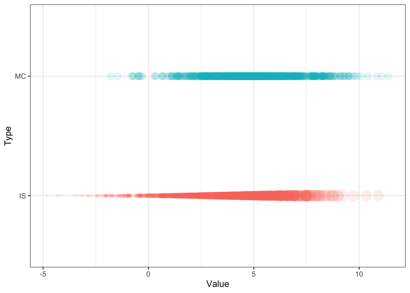
Figure 5.2: Standard Monte Carlo samples (top) and weighted samples from importance sampling (bottom).
We can generalize the importance sampler for cases where we have information only about a function that is proportional to the target distribution, i.e. \(p(\XX) = \frac {\rho(\XX)}{Z}\) where \(\rho(\XX)\) is known but \(Z = \int \rho(\XX) \ud \XX\) is not. The formulation of the target distribution becomes
\[ \begin{aligned} p(\XX) &= \frac {\rho(\XX)}{Z} \\ &= \frac {\rho(\XX)}{q(\XX)} \frac {q(\XX)}{Z} \\ &= W(\XX) \frac {q(\XX)}{Z}, \\ \end{aligned} \]
where \(W(\cdot) = \frac{\rho(\cdot)}{q(\cdot)}\) is the unnormalized (importance) weight function. With the samples drawn from \(q(\XX)\), this set-up allows for the following estimations:
\[ \begin{aligned} Z &= \int \rho(\XX) \ud \XX \\ &= \int \frac{\rho(\XX)}{q(\XX)} q(\XX) \ud \XX \\ &\approx \frac{1}{M} \sum_i W(\tilde \XX^{(i)}) \\ E_p[\varphi(\XX)] &= \int \varphi(\XX) W(\XX) \frac {q(\XX)}{Z} \ud \XX \\ &\approx \frac{1}{M} \sum_i \varphi(\tilde \XX^{(i)}) \frac {W(\tilde \XX^{(i)})}{\frac{1}{M} \sum_j W(\tilde \XX^{(j)})} \\ &= \sum_i \varphi(\tilde \XX^{(i)}) w^{(i)}, \end{aligned} \]
where \(w^{(i)} = \frac{W(\tilde \XX^{(i)})} {\sum_j W(\tilde \XX^{(j)})}\) represents the normalized weight. This idea can be further expanded to obtain a formal approximation of the target distribution
\[ p(\XX) \approx \sum_i w^{(i)} \delta_{\tilde \XX^{(i)}} (\XX), \]
where \(\delta_{\tilde \XX^{(i)}} (\XX)\) denotes the Dirac delta function centered at \(\tilde \XX^{(i)}\).
Essentially, in the IS framework, approximation of expectations are achieved by using weighted samples \((w^{(1)}, \tilde \XX^{(1)}), \ldots, (w^{(M)}, \tilde \XX^{(M)})\) when performing the Monte Carlo integration. This is an appealing approach to the state estimation problem, as this set-up can be applied to the approximation of the conditional distribution \(p(\XX_{0:t} \mid \YY_{0:t})\). However, it is important to note that the importance sampler becomes susceptible to computational break-down as time increases. This is because, for every time step with a new observation \(Y_{t+1}\), it requires recomputation of the weights over the entire trajectory \(\XX_{0:t+1}\) (Doucet, Freitas, and Gordon 2001). Such a drawback underlines the need for a modification in the importance sampling operation.
5.2.3 Sequential Importance Sampling
To address the aforementioned issue of increasing computational complexity, we aim to build a sequential approximation method within the importance sampling framework. Firstly, we consider a proposal distribution that has the following recursive structure:
\[ \begin{aligned} q(\XX_{0:T}) &= q(\XX_{0:(T-1)}) q(X_t \mid \XX_{0:(T-1)}) \\ &= q(X_0) \prod^T_{t=1} q(X_t \mid \XX_{0:(t-1)}). \end{aligned} \]
This allows to sample the trajectory \(\tilde \XX^{(i)}_{0:T} \sim q(X_{0:T})\) by sampling \(\tilde X_0^{(i)} \sim q(X_0)\) and \(\tilde X_t^{(i)} \sim q(X_t \mid \tilde \XX^{(i)}_{0:(t-1)})\) for \(t = 1, \ldots, T\).
For example, suppose we have the samples \(\{ \tilde X^{(i)}_0 \}\) with their associated weights \(\{ W(\tilde X^{(i)}_0) \}\) at time 0, and aim to approximate the target distribution \(p(\XX_{0:1})\). Since the samples at time 0 are already available, we only sample \(\tilde X^{(i)}_1 \mid \tilde X^{(i)}_0 \sim q(X_1 | \tilde X^{(i)}_0)\). Then, the weight function at time 1 can be decomposed as
\[ \begin{aligned} W(\XX_{0:1}) &= \frac {\rho(\XX_{0:1})} {q(\XX_{0:1})} \\ &= \frac {\rho(X_0)} {q(X_0)} \frac {\rho(\XX_{0:1})} {\rho(X_0) q(X_1 |X_{0})} \\ &= W(X_0) \cdot \alpha(\XX_{0:1}), \\ \end{aligned} \]
where \(\alpha(\XX_{0:1})\) is referred to as the incremental weight at time 1. The normalized weights at time 1 is proportional to the product of the normalized weights at time 0 and the incremental weight at time 1,
\[ \begin{aligned} w^{(i)}_1 \propto w^{(i)}_0 \cdot \alpha(\tilde \XX^{(i)}_{0:1}), \end{aligned} \]
which can be used for approximating the target distribution and the expectations. Using this logic, it is easy to prove that this sequential update of weights holds for a general case of \(W(\XX_{0:t}) = W(\XX_{0:(t-1)}) \cdot \alpha(\XX_{0:t})\).
From this, the Sequential Importance Sampling (SIS) algorithm can be constructed:
- At time \(t = 0\)
- Sample \(\tilde X^{(i)}_0 \sim q(X_0)\).
- Calculate the unnormalized weights \(W(\tilde X^{(i)}_0)\).
- Normalize the weights \(w^{(i)}_0 \propto W(\tilde X^{(i)}_0)\).
- At time \(t \ge 1\)
- Sample \(\tilde X_t^{(i)} \sim q(X_t \mid \tilde \XX^{(i)}_{0:(t-1)})\).
- Calculate the unnormalized weights \(W(\tilde \XX^{(i)}_{0:t}) = W(\tilde \XX^{(i)}_{0:(t-1)}) \cdot \alpha(\tilde \XX^{(i)}_{0:t})\).
- Normalize the weights \(w^{(i)}_t \propto W(\tilde \XX^{(i)}_{0:t})\).
The sequential update of weights provides a solution to the computational burden of the standard IS method, as each iteration is bounded by a fixed level of computational complexity. However, SIS is nonetheless vulnerable to other problems inherent to the IS framework, such as the exponential growth of variability in the estimates. An intuitive example of such a phenomenon is presented by Doucet and Johansen (2012).
One adverse implication of the SIS framework is weight degeneracy, which refers to a scenario where all but a very few samples have negligible weight. This leads to an unreliable approximation of the target distribution as only a small number of samples are involved in the calculation of the estimates. To address this problem, we need to include a remedial step to the SIS algorithm.
5.2.4 Sequential Importance Resampling
To battle the weight degeneracy, we can resample the trajectories \(\{ \tilde \XX^{(i)}_{0:t} \}\) according to probability \(w^{(i)}\) and set the weight of the newly selected trajectories equally to \(\frac 1 M\). This allows us to discard trajectories with low weights and replenish with those with higher weight.
Resampling of trajectories is equivalent to sampling the number of offspring trajectories from a multinomial distribution with weight as probability, \(M^{(1:M)}_{off} \sim \operatorname{Multinomial} (M, w^{(1:M)})\). Then the approximation of the target distribution after resampling becomes
\[ p(\XX) \approx \sum_i \frac{M^{(i)}}{M} \delta_{\tilde \XX^{(i)}} (\XX), \]
and \(E[M^{(i)} \mid w^{(1:M)}] = Mw^{(i)}\), hence an unbiased estimate of the IS approximation of the target distribution.
It is important to keep in mind that, although resampling provides major advantages on maintaining the balance of the weights, it nonetheless injects additional variance to the approximations (Chopin 2004). A major consequence of frequent resampling is faster sample impoverishment, which refers to a reduction in the number of distinct samples. To mitigate this problem, we consider a popular method of establishing the resampling criterion by the effective sample size (ESS), given by
\[ ESS = \frac{M}{1 + \frac{\var(w)} {\bar w^2}}. \]
A typical usage is to calculate the ESS at each time step, and resample the trajectories when the ESS drops to or below a certain threshold, determined by \(\lambda M, \lambda \in [0,1]\).
With this modification, we can define the Sequential Importance Resampling (SIR) algorithm:
- At time \(t = 0\)
- Sample \(\tilde X^{(i)}_0 \sim q(X_0)\).
- Calculate the unnormalized weights \(W(\tilde X^{(i)}_0)\).
- Normalize the weights \(w^{(i)}_0 \propto W(\tilde X^{(i)}_0)\).
- If \(ESS_0 \le \lambda M\),
- Resample \(\{w^{(i)}_0, \tilde X^{(i)}_0 \}\) and obtain \(M\) trajectories \(\{\frac 1 M, \bar X^{(i)}_0 \}\).
- At time \(t \ge 1\)
- Sample \(\tilde X_t^{(i)} \sim q(X_t \mid \tilde \XX^{(i)}_{0:(t-1)})\).
- Calculate the unnormalized weights \(W(\tilde \XX^{(i)}_{0:t}) = W(\tilde \XX^{(i)}_{0:(t-1)}) \cdot \alpha(\tilde \XX^{(i)}_{0:t})\).
- Noramlize the weights \(w^{(i)}_t \propto W(\tilde \XX^{(i)}_{0:t})\).
- If \(ESS_t \le \lambda M\),
- Resample \(\{w^{(i)}_t, \tilde \XX^{(i)}_{0:t} \}\) and obtain \(M\) trajectories \(\{\frac 1 M, \bar \XX^{(i)}_{0:t} \}\).
Evidently, if \(\lambda = 0\), there will be no resampling step in any of the iterations, which is essentially the SIS algorithm; on the other hand, if \(\lambda = 1\), there will always be a resampling step and will thus become a greedy SIR algorithm. The implications of the choice of \(\lambda\) are further explored in the Worked Example section.
5.3 Particle Filter
5.3.1 Intuitive formulation
In order to demonstrate the workings of a particle filter step-by-step, we continue the robot localization example from the previous example. An application of particle filtering to this task in practice can be found at Fox et al. (2001). A picture is worth a thousand words, so we borrow an animation by the same author depicting this exact phenomenon.
In this depiction, we can see an initial state with particles uniformly dispersed throughout the map, each representing a candidate location for the robot. As described in this example, we imbue the robot with a limited form of vision (in this exact example, sonar) that reveals some indirect information about its location. The blue lines indicate the purported distance implied by the sonar return in that direction from the robot.
Using these sonar measurements, we can sample from the posterior and generate an importance weight for each particle. Using this additional information, we can resample these particles according to these weights, leading to particles congregating in likely robot positions.
As the green dot is the most likely position of the robot, we find that it jumps around at the outset. Since the robot is on the move and acquiring new data from a different position over time, the particle filter is increasingly able to refine the position estimate. Note that there are some isolated but also very concentrated pockets of particles that remain in intermediate iterations; this demonstrates the multi-modality of the distribution that hinders other methods such as Kalman filters. Additionally, note that the blue lines do not always coincide with the map’s distances even when the robot is well-localized; this is the noisy nature of the measurement system. In practice, sonar can lead to errant readings due to echos, interference, and absorption.
A detailed explanation of the precise workings of particle filtering follows. We encourage the reader to bear this illustrative example in mind while handling the notation as it very intuitively distinguishes the nature of the system and measurement models.
5.3.2 Definition and Algorithm
As we have established the fundamentals of the importance sampling, it is easy to understand how the SIR algorithm can be applied to the cases of state-space models. Essentially, we can set the distributions according to the formulation of the IS framework:
\[ p(\XX) = p(\XX_{0:t} \mid \YY_{0:t}) \\ \rho(\XX) = p(\XX_{0:t}, \YY_{0:t}) \\ Z = p(\YY_{0:t}). \]
As seen previously, we only need to select \(q(X_t \mid \XX_{0:(t-1)})\) since the proposal distribution can be defined recursively. This gives
\[ \begin{aligned} q(X_t \mid \XX_{0:(t-1)}) \implies& q(X_t \mid \XX_{0:(t-1)}, \YY_{1:t}) \\ = \; & q(X_t \mid X_{t-1}, Y_t) \\ = \; & \frac{g(Y_t \mid X_t) f(X_t \mid X_{t-1})} {p(Y_t \mid X_{t-1})}. \end{aligned} \]
The importance weight function can be derived as the following:
\[ \begin{aligned} W(\XX_{0:t}) &= W(\XX_{0:(t-1)}) \frac{p(\XX_{0:t}, \YY_{0:t})}{p(\XX_{0:(t-1)}, \YY_{0:(t-1)}) p(X_t \mid X_{t-1}, Y_t)} \\ &= W(\XX_{0:(t-1)}) \frac{p(X_t, Y_t\mid \XX_{0:(t-1)}, \YY_{0:(t-1)})}{p(X_t \mid X_{t-1}, Y_t)} \\ &= W(\XX_{0:(t-1)}) \frac{p(X_t, Y_t\mid X_{t-1})}{p(X_t \mid X_{t-1}, Y_t)} \\ &= W(\XX_{0:(t-1)}) \cdot p(Y_t \mid X_{t-1}). \end{aligned} \]
The incremental weight function in this case is \(\alpha(\XX_{0:t}) = p(Y_t \mid X_{t-1})\), from which it may not be possible to sample. Instead, we use
\[ \alpha(\XX_{0:t}) = \frac{g(Y_t \mid X_t) f(X_t \mid X_{t-1})} {q(X_t \mid X_{t-1}, Y_t)}. \]
After these adaptations to the SIR algorithm, the Particle Filtering algorithm can be constructed.
The Particle Filtering algorithm:
- At time \(t = 0\)
- Sample \(\tilde X^{(i)}_0 \sim q(X_0 \mid Y_0)\).
- Calculate the unnormalized weights \(W(\tilde X^{(i)}_0) = \frac{\pi(\tilde X^{(i)}_0) g(Y_0 \mid \tilde X^{(i)}_0)}{q(\tilde X^{(i)}_0 \mid Y_0)}\).
- Normalize the weights \(w^{(i)}_0 \propto W(\tilde X^{(i)}_0)\).
- If \(ESS_0 \le \lambda M\),
- Resample \(\{w^{(i)}_0, \tilde X^{(i)}_0 \}\) and obtain \(M\) trajectories \(\{\frac 1 M, \bar X^{(i)}_0 \}\).
- At time \(t \ge 1\)
- Sample \(\tilde X_t^{(i)} \sim q(X_t \mid \tilde \XX^{(i)}_{0:(t-1)}, Y_t)\).
- Calculate the unnormalized weights \(W(\tilde \XX^{(i)}_{0:t}) = W(\tilde \XX^{(i)}_{0:(t-1)}) \cdot \alpha(\tilde \XX^{(i)}_{0:t})\), where \(\alpha(\tilde \XX^{(i)}_{0:t}) = \frac{g(Y_t \mid \tilde X^{(i)}_t) f(\tilde X^{(i)}_t \mid \tilde X^{(i)}_{t-1})} {q(\tilde X^{(i)}_t \mid \tilde X^{(i)}_{t-1}, Y_t)}\).
- Noramlize the weights \(w^{(i)}_t \propto W(\tilde \XX^{(i)}_{0:t})\).
- If \(ESS_t \le \lambda M\),
- Resample \(\{w^{(i)}_t, \tilde \XX^{(i)}_{0:t} \}\) and obtain \(M\) trajectories \(\{\frac 1 M, \bar \XX^{(i)}_{0:t} \}\).
5.3.3 Worked example
5.3.3.1 Bootstrap filter to noisy random-walk
The bootstrap filter, the most basic and intuitive version of particle filter, is considered in this example. Proposed by Gordon, Salmond, and Smith (1993), bootstrap filter is a special version of the particle filter with a proposal distribution \(q(X_t \mid X_{t-1}, Y_t) = f(X_t \mid X_{t-1})\). This leads to a simplified calculation of the importance weight of \(W(\tilde \XX^{(i)}_{0:t}) = W(\tilde \XX^{(i)}_{0:(t-1)}) \cdot g(Y_t \mid \tilde X^{(i)}_t)\).
Suppose we have a simple noisy random-walk model:
\[ X_0 \sim \N(0, \sigma_{rw}^2) \\ X_t = X_{t-1} + \omega_t, \quad \omega_t \sim \N(0, \sigma_{rw}^2) \\ Y_t = X_t + \epsilon_t, \quad \epsilon_t \sim \N(0, \sigma_{obs}^2). \\ \]
Then, we have \(X_t \mid X_{t-1} \sim \N(X_{t-1}, \sigma_{rw}^2)\) and \(Y_t \mid X_t \sim \N(X_t, \sigma_{obs}^2)\), from which we can define the incremental weight \(\alpha(\tilde \XX^{(i)}_{0:t}) = g(Y_t \mid \tilde X^{(i)}_t) = \phi(Y_t; \tilde X^{(i)}_t, \sigma_{obs})\), where \(\phi(\cdot)\) represents the normal density. We also approximate the mean of the particles at each iteration to compare with the actual value of the hidden state. The following code executes the bootstrap filtering operation5.
# Toy example of the bootstrap filter.
set.seed(1234)

# Parameters set-up.
sigma_rw <- 2
sigma_obs <- 3
len <- 100 # length of data
M <- 100 # number of particles
lambda <- 0.5 # resampling criterion coefficient

# Generate data.
x <- cumsum(rnorm(len, 0, sigma_rw))
y <- x + rnorm(len, 0, sigma_obs)

# Variable set-up.
part_traj <- # particle trajectory
  weight <- # importance weight
  matrix(rep(NA, len * M), ncol = M)
avg <- rep(NA, len) # the approximated average

# Initialize.
part_traj[1, ] <- rnorm(M, 0, sigma_rw)
weight[1, ] <- 1/M
avg[1] <- mean(part_traj[1, ])

# Particle filtering algorithm.
for (t in 2:len) {
  # Propagate particles according to X_t | X_{t-1}.
  part_traj[t, ] <- part_traj[t-1, ] + rnorm(M, 0, sigma_rw)

  # Calculate importance weights and normalize.
  w <- weight[t-1,] * dnorm(y[t], part_traj[t,], sigma_obs)
  weight[t,] <- w / sum(w)
  avg[t] <- sum(weight[t,] * part_traj[t,]) # the weighted expectation

  # Resampling criterion by effective sample size.
  ess <- M / (1 + var(weight[t,]) / mean(weight[t,]) ^ 2)
  if (ess <= lambda * M) {
    # Resample the particles with replacement.
    s <- sample(M, M, replace = TRUE, prob = w)
    part_traj <- part_traj[,s]
    weight[t,] <- 1 / M # reset weight
  }
}
The result is shown in Figure 5.3.
require(ggplot2)

gg_df <- data.frame("Time" = 1:len, "Observed" = y, "Hidden" = x, "Mean" = avg)
shapes <- c(NA, NA, 16)
colors <- c("black", "red", "grey")

ggplot(gg_df, aes(x = Time)) + theme_bw() + labs(x = "Time", y = "Value") +
  geom_point(aes(y = Observed, color = "Observed")) +
  geom_line(aes(y = Hidden, color = "Hidden")) +
  geom_line(aes(y = Mean, color = "Mean")) +
  scale_color_manual("Data", values = colors,
                     guide = guide_legend(override.aes = list(
                       linetype = c("solid", "solid", "blank"),
shape = shapes))) 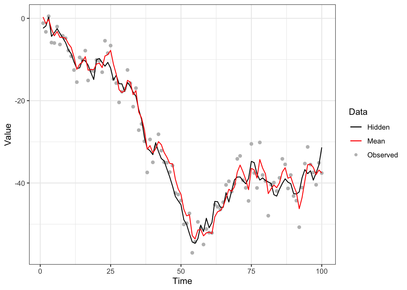
Figure 5.3: Bootstrap filter to noisy random-walk model with system model (black line), measurement model (grey points) and approximated mean (red line).
5.3.3.2 Particle filter to nonlinear dynamical model
A more sophisticated example is the nonlinear dynamical model presented by Cappé, Moulines, and Ryden (2007), with the state-space model
\[ X_t = \underbrace {\alpha X_{t-1} + \beta \frac{X_{t-1}}{1+X_{t-1}^2} + \gamma \cos(\omega t) }_{\mu_t(X_{t-1})} + \sigma_X U_t \\ Y_t = \eta X_t^2 + \sigma_Y V_t \\ U_t, V_t \iid \N(0,1). \]
For this filtering problem, instead of the bootstrap proposal \(q(X_t \mid X_{t-1}, Y_t) = f(X_t \mid X_{t-1})\), we employ a bivariate normal approximation of the proposal distribution \[ q(X_t \mid X_{t-1}, Y_t) \propto \exp \left \{ - \frac {[X_t - \mu_t(X_{t-1})]^2}{2 \sigma_X^2} - \frac {[Y_t - \eta X_t^2]^2}{2 \sigma_Y^2} \right \} \] by mode-matching. That is, since \(\ell (X_t) = \log q(X_t \mid X_{t-1}, Y_t)\) is a quartic polynomial in \(X_t\) with at most two modes, the maxima \(\hat X_t = \arg \max_{X_t} q(X_t \mid X_{t-1}, Y_t)\) can be found by the roots of the cubic polynomial \(\frac{\ud} {\ud X_t} \ell (X_t)\). Then, we build a “mode-quadrature” proposal with a Normal distribution
\[ \N \left ( \hat X_t, Q(\hat X_t) \right ), \quad Q(\hat X_t) = -\left [ \frac{\ud^2} {\ud X_t^2} \ell (\hat X_t) \right ]^{-1} \] if only one mode exists, and with a mixture Normal distribution
\[ \N \left ( \hat X_{t,z}, Q(\hat X_{t,z}) \right ), \quad z \sim \operatorname {Multinomial}(1, \rrh) \] if two modes exist, where \(\rrh \propto \left[(\ell (\hat X_{t,1}) - \ell (\hat X_{t,2})) \sqrt{\frac{Q(\hat X_{t,1})} {Q(\hat X_{t,2})}}, 1 \right]\). Figure 5.4 shows the approximation of proposal distribution against the target distribution, scaled to each other.
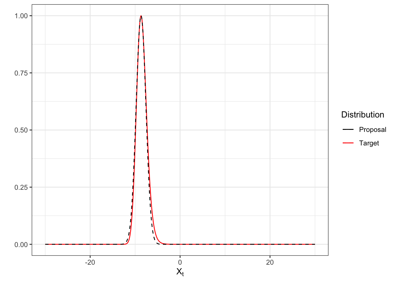
Figure 5.4: Bivariate normal approximation (black dashed curve) of the target distribution (red solid curve) by solving cubic root, scaled to each other.
With this, we can implement the particle filter to the model. The following code executes the particle filtering operation6.
# Example of particle filter to nonlinear dynamical model.
# Reproduced from course notes by Martin Lysy.
normalize <- function(x) {x/sum(x)}
set.seed(1234)

# Parameter set-up.
theta <- c(alpha = .5, beta = 25, gamma = 8, omega = 1.2, eta = .05,
           sigX = sqrt(10), sigY = 1) # model parameter
nObs <- 30 # number of observations
nPart <- 50 # number of particles
lambda <- 0.1 # threshold coefficient

# Generate data.
X0 <- rnorm(1, sd = theta["sigX"]) # initial state
nd_data <- rnldyn(nObs, X0, theta) # generate hidden and observed data
Yt <- nd_data[,2]

# Variable set-up.
Particles <- matrix(NA, nPart, nObs) # particles
logWeights <- matrix(NA, nPart, nObs) # log-weights
propParams <- matrix(list(), nPart, nObs) # parameters of proposal
avg <- rep(NA, nObs) # the approximated average

# Initialize particles and assign log-weights.
Particles[,1] <- rnorm(nPart, sd = theta["sigX"])
logWeights[,1] <- dnorm(Yt[1],
                        mean = theta["eta"] * Particles[,1]^2,
                        sd = theta["sigY"],
                        log = TRUE)
avg[1] <- sum(normalize(exp(logWeights[,1]))*Particles[,1])

# Mixture normal becomes univariate normal.
propParams[,1] <- list(cbind(mu = c(0, 0),
                             sig = c(theta["sigX"], Inf),
                             rho = c(1, 0)))

# Particle filtering algorithm.
for (iStep in 2:nObs) {
  for (iPart in 1:nPart) {
    # Calculate parameters of the mode-quadrature proposal.
    qpar <- prop_par(t1 = iStep - 1,
                     Y1 = Yt[iStep],
                     X0 = Particles[iPart, iStep - 1],
                     theta = theta)
    # Sample from mode-quadrature proposal.
    part <- rnmix(1, qpar[, "mu"], qpar[, "sig"], qpar[, "rho"])
    # Weight increment
    lw <- nldyn_ltarg(X1 = part,
                      t1 = iStep - 1,
                      Y1 = Yt[iStep],
                      X0 = Particles[iPart, iStep - 1],
                      theta = theta) # this is the g(Y_t | X_t) f(X_t | X_{t-1})
    lw <- lw - dnmix1(part, qpar[, "mu"], qpar[, "sig"], qpar[, "rho"],
                      log = TRUE) # this is the q(X_t | X_{t-1}, Y_t)

    # Store values
    Particles[iPart, iStep] <- part
    logWeights[iPart, iStep] <- logWeights[iPart, iStep - 1] + lw
    propParams[[iPart, iStep]] <- qpar
  }

  normWeight <- normalize(exp(logWeights[,iStep]))
  avg[iStep] <- sum(normWeight*Particles[,iStep])

  # Resampling criterion by effective sample size.
  ess <- nPart / (1 + var(normWeight)/mean(normWeight)^2)
  if (ess <= lambda*nPart) {
    # Resample the particles with replacement.
    s <- sample(nPart, nPart, replace = TRUE, prob = normWeight)
    Particles <- Particles[s,]
    logWeights[,iStep] <- log(1/nPart) # reset weight
  }
}
The result of this particle filter is illustrated in Figure 5.5.
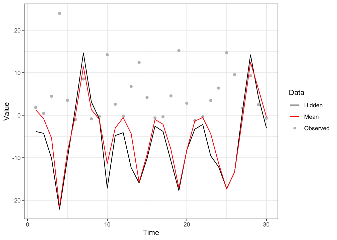
Figure 5.5: Particle filter with mode-quadrature proposal to nonlinear dynamical model with system model (black line), measurement model (grey points) and approximated mean (red line).
More examples of the particle filter are presented in the pomp package section.
5.3.3.3 Weight degeneracy
As discussed in the Sequential Importance Sampling section, weight degeneracy occurs when the particles are never resampled in the algorithm and as a result, provides an inadequate representation of the target distribution. In order to investigate weight degeneracy, we revisit the noisy random-walk example. Figure 5.6 shows the bootstrap filter with no resampling step, which is essentially when \(\lambda = 0\).
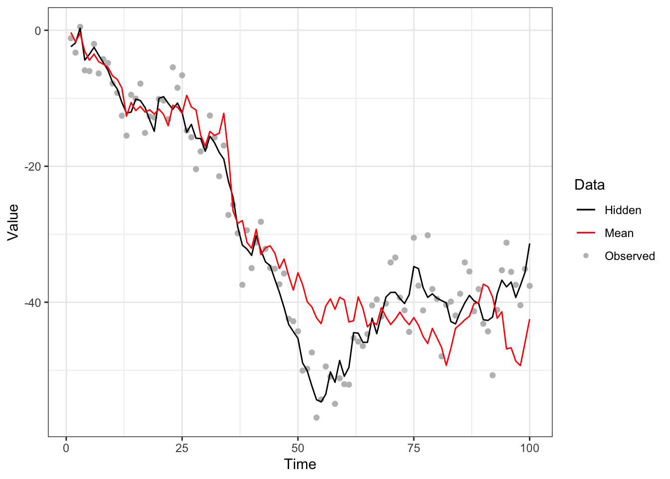
Figure 5.6: Bootstrap filter to noisy random-walk with no resampling step with system model (black line), measurement model (grey points) and approximated mean (red line).
It is clear that the approximation of the mean is inaccurate relative to Figure 5.3, due to the decreasing number of particles with significant weight. This can be better visualized by the histograms of the particle weights at differet time steps, illustrated in Figure 5.7. We observe that, at time 30, one particle has dominant weight and the rest have weights near zero.
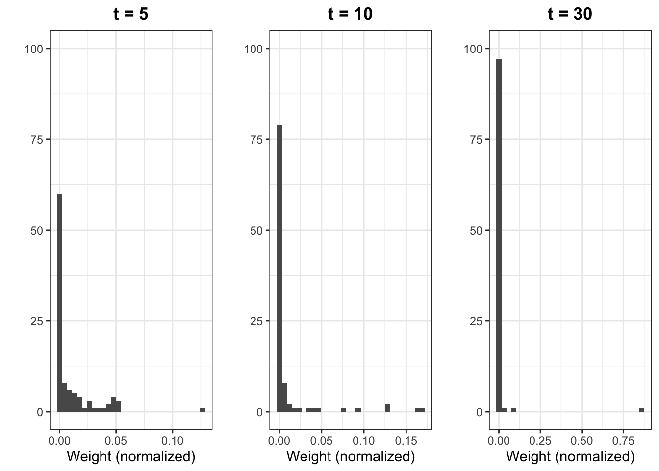
Figure 5.7: Histograms of particle weights at time 5 (left), 10 (center) and 30 (right).
5.3.3.4 Sample impoverishment
A major issue caused by resampling was introduced in the Sequential Importance Resampling section, namely sample impoverishment. Again, we use the noisy random-walk example to illustrate this phenomenon. It is presented in Figure 5.8 the association between the resampling frequency and the rate at which number of distinct particles decreases.
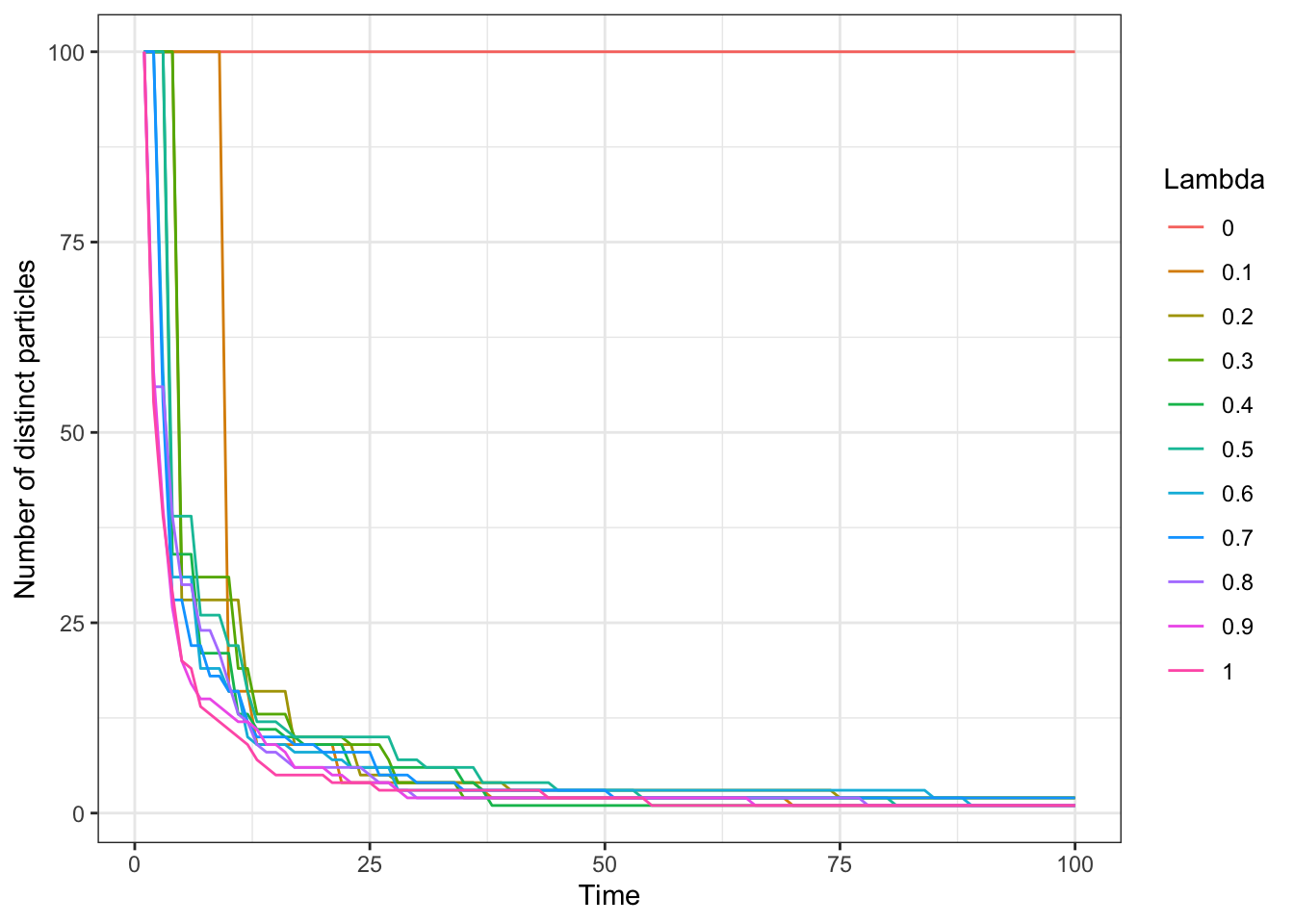
Figure 5.8: Number of distinct particles across time for choice of threshold coefficient.
While it is true that a lower threshold results in a slower impoverishment of samples, the number of distinct particles eventually decays as time passes, regardless of the choice of \(\lambda\) if \(\lambda > 0\). Figure 5.8 re-emphasizes this inevitable consequence of the SIR framework, from which the particle filter was derived.
5.4 Parameter Estimation
When the state-space model as described in [State-space model] has state transition and observation distributions governed by some latent but fixed parameters, say \(\theta\) in some domain \(\Theta\), we may perform particle MCMC. In such a case, we add a subscript \(\theta\) to the state transition equation \(f_\theta\) and the observation equation \(g_\theta\).
When \(\theta\) is a unknown parameter of interest, we may impose a suitable prior \(p(\theta)\) and perform Bayesian inference for the joint distribution given as:
\[ p(\theta \mid\YY) \propto \int {p(\theta) p(\XX,\YY\mid\theta) \ud\XX} \] Particle MCMC methods can be used for Bayesian estimation of state-space models that go beyond the case of linear or Gaussian SSMs (for which tractable or regular MCMC solutions exist.) In these cases, \(p(\theta\mid\YY)\) lacks a closed form and is difficult to work with exactly.
The following subsections briefly introduce some particle variations on MCMC methods.
5.4.1 Particle independent Metropolis-Hastings (PIMH)
Under usual Metropolis-Hastings, we would need to choose a proposal distribution \(q_\theta(\XX_{0:T}\mid\YY_{0:T})\) to draw candidate values of \(\XX_{0:T}\) which we may accept or reject according to an acceptance ratio. The particle variation follows from using the particle filter approximation to the posterior density as the proposal distribution. The following briefly lists the steps to perform this type of PMCMC:
- Perform particle filtering to draw a sample \(\tilde\XX\) and estimate the marginal likelihood of the observed values \(\hat{p}_\theta(\YY)\)
- Do step 0 to draw a candidate sample \(\tilde\XX^*\) with corresponding estimate \(\hat{p}_\theta(\YY)^*\).
- Compute the acceptance probability \(\min\left\lbrace 1, \frac{\hat p_\theta(\YY)^*}{\hat p_\theta(\YY)}\right\rbrace\).
- If accept, update \(\tilde\XX\to\tilde\XX^*\) and \(\hat{p}_\theta(\YY)\to\hat{p}_\theta(\YY)^*\).
- Take the current \(\XX\) as a sample, and return to step 1.
This yields a sequence of samples of \(\XX\), and exhibits desirable properties under certain assumptions; see Andrieu, Doucet, and Holenstein (2010) for more details.
5.4.2 Particle Marginal Metropolis-Hastings (PMMH)
While PIMH allows us to draw samples of \(\XX\), we may also wish to perform some sort of inference on the latent hyperparameter \(\theta\). For this, we may turn to PMMH whereby both the latent \(\XX\) and \(\theta\) are updated jointly. To ease this process, we may decompose the joint proposal distribution; first drawing a candidate \(\theta^*\) from a marginal proposal \(q\) and then drawing a candidate \(\XX^*\) from a conditional distribution \(p_{\theta^*}\). The PMMH process is summarized below:
- Initialize \(\theta\) arbitarily, perform particle filtering to generate a sample \(\tilde\XX\sim \hat{p}_\theta(\XX\mid\YY)\), and estimate the marginal likelihood \(\hat{p}_\theta(\YY)\).
- Draw \(\theta^*\) from \(q_\theta\).
- Run particle filtering to draw a candidate \(\XX^*\) and compute the new candidate marginal likelihood \(\hat{p}_{\theta^*}(\YY)^*\).
- Compute the acceptance probability \(\min\left\lbrace 1, \frac{\hat p_{\theta^*}(\YY)^*p(\theta^*)}{\hat p_\theta(\YY)p(\theta)}\frac{q(\theta\mid\theta^*)}{q(\theta^*\mid\theta)}\right\rbrace\).
- If accept, update \(\theta\to\theta^*\), \(\tilde\XX\to\tilde\XX^*\) and \(\hat{p}_\theta(\YY)\to\hat{p}_\theta(\YY)^*\).
- Take the current \(\XX\) and \(\theta\) as a sample, and return to step 1.
For a worked example in R using the pomp package, see the pomp package section.
5.4.3 Particle Gibbs sampler
For completeness, we mention the particle Gibbs, whereby the update on \(\XX\) and \(\theta\) occur sequentially instead of jointly. This avoids the need to craft an appropriate proposal distribution on \(\theta\) as required in PMMH. For a precise description of the particle Gibbs sampler, see Section 2.4.3 and 4.5 in Andrieu, Doucet, and Holenstein (2010).
5.5 Practical Software Implementations
There are a multitude of software implementations for particle filtering. For pedagogical purposes, we have demonstrated particle filters and PMCMC using the pomp package, which exposes itself to the end user entirely in terms of R code. This provides an easy introductory access to Bayesian computation for R users who are not yet comfortable with C++ to delve into more capable and performant packages. We briefly mention the plethora of alternative software packages capable of working with particle filters, such as msde, LibBi (and its R wrapper rbi), SMCTC (and its R wrapper RcppSMC), and vSMC (no R wrapper available yet).
5.6 pomp package
Here, we demonstrate the usage of the pomp package (King et al. 2020) as hosted on CRAN for the R programming language. We attribute the entirety of the example to the author’s vignette at https://kingaa.github.io/pomp/vignettes/pompjss.pdf and upgrade guide found at https://kingaa.github.io/pomp/vignettes/upgrade_guide.html but with some stylistic changes for understanding. Be careful with the above reference sources as the syntax has changed between version 1 and version 2 of the package. Moreover, you will need to be able to compile from source for your platform. (This means installing Rtools for Windows!)
require(pomp)
require(tidyverse)
5.6.1 Specification
We follow the Gompertz model specification of a state-space model which describes a population over time with measurement error. In particular, we have the following state transition equation:
\[ X_{t+\Delta t}=K^{(1-e^{-r\Delta t})} \times X_t^{e^{-r\Delta t}}\times \varepsilon_t \] Note that in this case the noise is not additive but multiplicative, and that we allow an arbitrary step size \(\Delta t\). For our intents and purposes, this does not pose an issue. Moreover, we specify the state transition error distribution as \(\log\varepsilon_t \overset{\text{iid}}{\sim}\N(0,\sigma^2)\). In R, we write express this as the following function:
gompertz_state_transition <- function (X, r, K, sigma, delta.t, ...) {
  eps_t <- exp(rnorm(1, 0, sigma))
  S     <- exp(-r * delta.t)
  X_new <- K^(1 - S) * X^S * eps_t
  return(c(X = X_new))
}
The measurement system is a noisy observation of the true population with observations \(\log{Y_t}\sim \N(\log{X_t}, \tau^2)\).
gompertz_observation <- function (X, tau, ...) {
  Y_obs <- rlnorm(1, log(X), tau)
  return(c(Y = Y_obs))
}
Next, we define the conditional distribution \(g(Y_t\mid X_t)\), which as stated above, is the lognormal distribution with parameters \(\log{X_t}\) and \(\tau\):
\[ g(Y_t\mid X_t) = \frac{1}{Y_t\sqrt{2\pi\tau^2}} \exp{\left(-\frac{(\log{Y_t}-\log{X_t})^2}{2\tau^2}\right)} \]
g_y_given_x <- function (X, tau, Y, log, ...) {
  return(dlnorm(Y, log(X), tau, log = log))
}
Finally, we implement a very simple function to initialize the system model at \(X_0\):
initialize_system_model <- function (X_0, ...) {
  return(c(X = X_0))
}
Since the state transition and observation equations depend on some yet unspecified parameters \(r\), \(K\), \(\sigma\), and \(\tau\), we make some reasonable initializations below. Furthermore, we initialize the system model \(X_0\) here as well.
\[ r = 0.1 \quad K = 1 \quad \sigma = 0.1 \quad \tau = 0.1 \quad X_0 = 1 \]
Armed with these pieces, we may call the simulate function to construct a
state-space model object. As mentioned before, we may choose to have our choice
of time steppings \(\Delta t\); for now, we will use the simplest case
\(\Delta t = 1\) up to \(T = 100\).
gompertz_ssm <- simulate(
  seed       = 12345,
  times      = 1:100,
  t0         = 0,
  rprocess   = discrete_time(gompertz_state_transition, delta.t = 1),
  rmeasure   = gompertz_observation,
  dmeasure   = g_y_given_x,
  rinit      = initialize_system_model,
  partrans   = parameter_trans(log = c("K", "r", "sigma", "tau")),
  paramnames = c("K", "r", "sigma", "tau"),
  params     = c(r = 0.1, K = 1, sigma = 0.1, tau = 0.1, X_0 = 1)
)
If all has gone well, we now have a single simulation run of the specified state-space model.
5.6.2 Particle Filter
We now perform state estimation using a standard particle filter with 1000 particles and resampling at every observation. While we set a seed here, the results tend to be consistent at least for this state-space model.
set.seed(123456)
pf_result <- pfilter(gompertz_ssm,
                     Np          = 1000,
                     filter.mean = TRUE,
                     filter.traj = TRUE)
We display below the true underlying latent system model, the observed measurement model, and the mean of the filtering distribution obtained from the above particle filter:
data.frame(Time            = gompertz_ssm@times,
           System          = gompertz_ssm@states[1,],
           Measurement     = gompertz_ssm@data[1,],
           "Filtered Mean" = pf_result@filter.mean[1,]) %>%
  pivot_longer(cols      = -1,
               names_to  = "Model",
               values_to = "Value") %>%
  ggplot(aes(x = Time, y = Value, colour = Model)) +
  geom_line() + facet_grid(Model ~ .)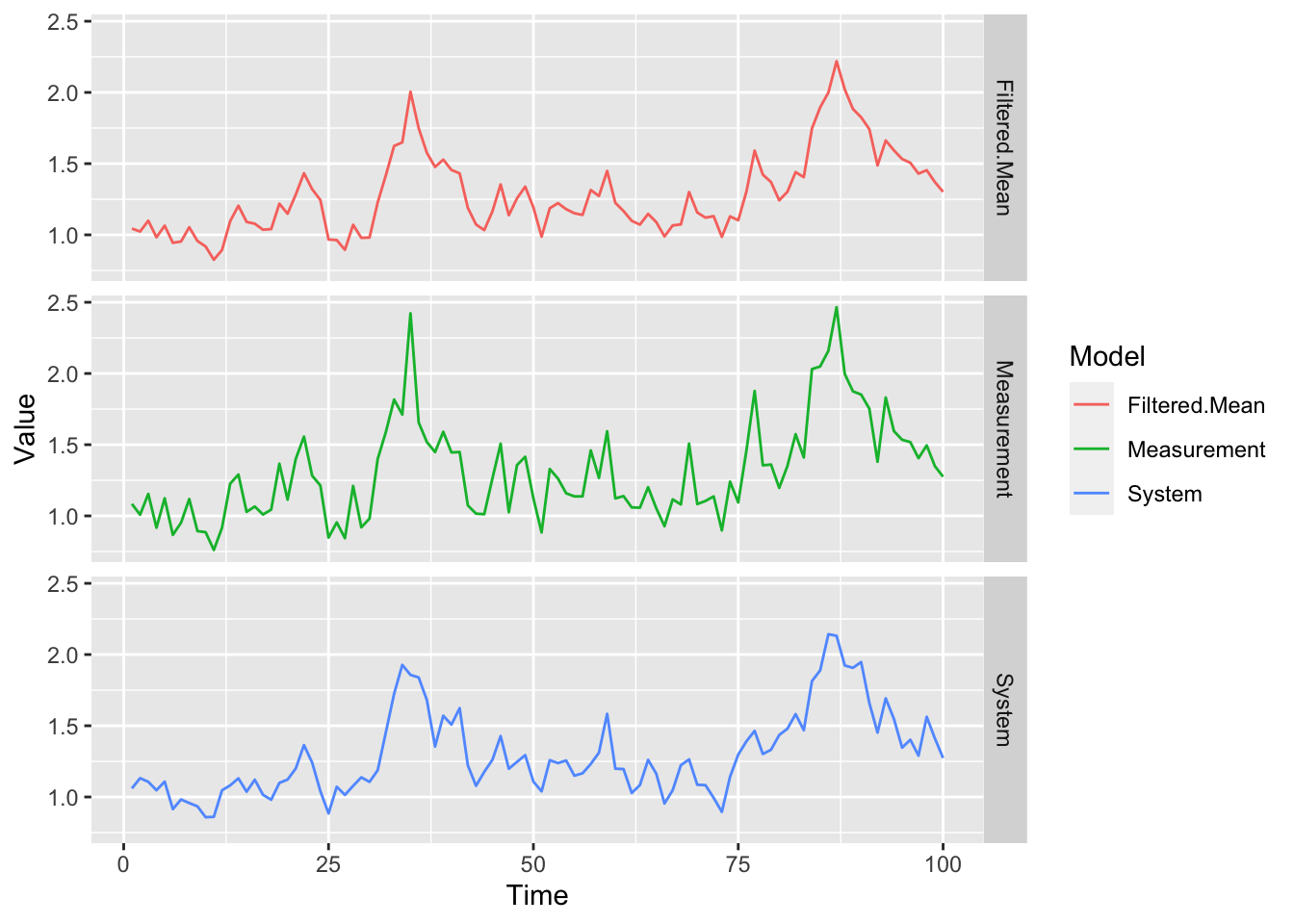
5.6.3 Particle MCMC - PMMH
Moreover, the pomp package offers the ability to run the PMMH algorithm described by Andrieu, Doucet, and Holenstein (2010). One caveat that pomp currently makes clear for this method is that the proposal density must be symmetric for the inference to be valid. Since our parameters are all non-negative, this poses a mild problem; for demonstration purposes, we simply choose very conservative proposal distributions for the parameters below to reduce the chance of a negative candidate value. The following proposal distributions are chosen, and are independent of each other:
\[ \begin{aligned} r^* &\sim\N(r,0.01^2) \\ K^* &\sim\N(r,0.1^2) \\ \sigma^* &\sim\N(r,0.01^2) \\ \tau^* &\sim\N(r,0.01^2) \\ X_0^* &\sim\N(r,0.1^2) \end{aligned} \] Finally, we impose a simple prior where all parameters independently follow a \(\operatorname{exp}(1)\) distribution:
\[ \pi(r,K,\sigma,\tau,X_0) = e^{-r}e^{-K}e^{-\sigma}e^{-\tau}e^{-X_0} \]
prior_density = function(log, r, K, sigma, tau, X_0, ...) {
  return(dexp(r, log = log) *
           dexp(K, log = log) *
           dexp(sigma, log = log) *
           dexp(tau, log = log) *
           dexp(X_0, log = log))
}
We also initialize the parameters away from the true value; we simply start at double the true values and allow the PMCMC algorithm to work its way down to the true values. For computational time reasons, we run a paltry 50 MCMC iterations; we recommend that you experiment with considerably higher values.
set.seed(12345)
pmcmc_result <- pmcmc(pf_result,
                      Nmcmc = 50,
                      dprior = prior_density,
                      params = c(r = 0.2, K = 2, sigma = 0.2, tau = 0.2, X_0 = 2),
                      proposal = mvn.diag.rw(c(r = 0.01, K = 0.1, sigma = 0.01, tau = 0.01, X_0 = 0.1)))

plot(pmcmc_result)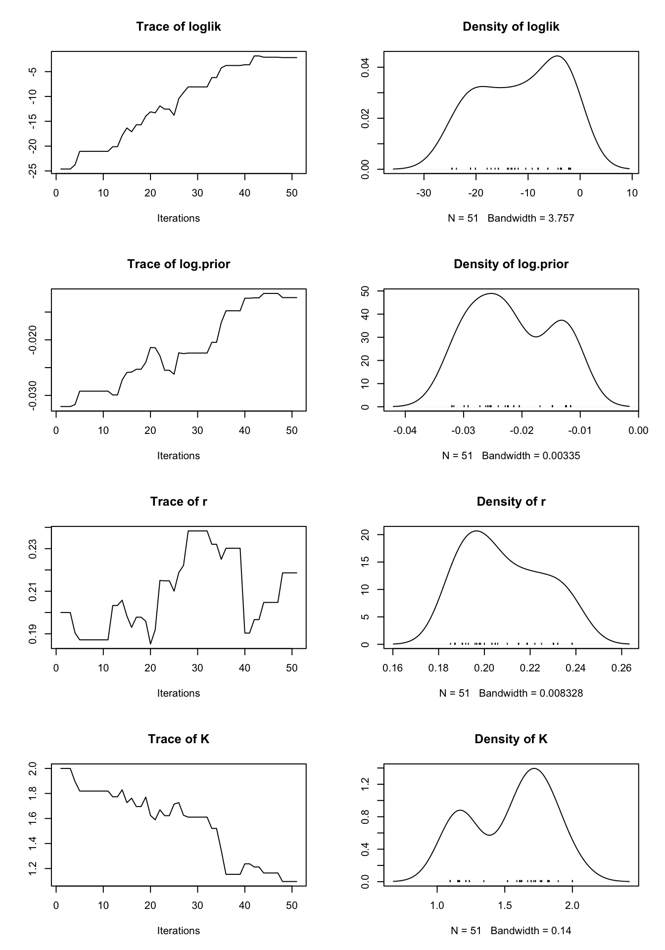
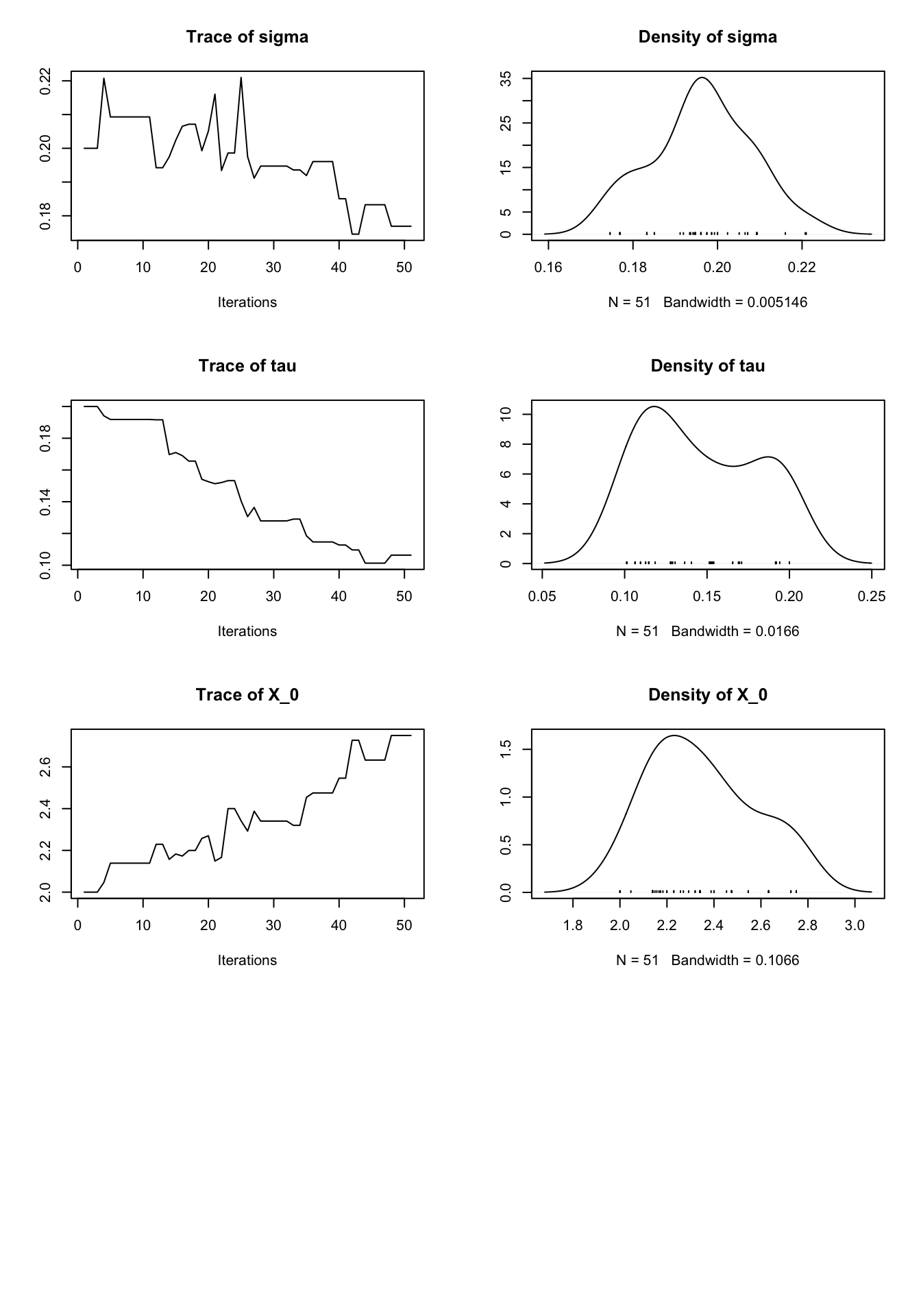
We can see in the above plot that many of the parameters descended towards their true values. Some unexpected behavior is seen, though we attribute this to the exceedingly low number of iterations. We encourage the reader to experiment with other possible state-space models and get some hands-on experience with the impact of the proposal distribution choice.