Chapter 7 Bayesian Non-parametrics
7.1 History
De Finetti’s theorem (De Finetti 1931) and Polya’s Urn are often used as starting points to facilitate a discussion of Bayesian non-parametric(BNP) methods. The theorem demonstrates that a fundamental relationship between \(\tx{iid}\) and exchangeable sequences exist and implies the existence of the rigorous mathematical basis for BNP that has developed since its discovery. Polya’s Urn provides a tactile demonstration of exchangeability and a basis for various approaches to considering the Dirichlet process.
7.1.1 Exchangeable Sequences of Random Variables
The first concept we consider is that of the exchangeable sequence of random variables. An exchangeable sequence of random variables may be finite or infinite in length and has a joint probability function that does not depend on the ordering of the events within it. No assumptions are made about the distribution of the sequence, or the independence of events in the sequence. It is important to note that while \(\tx{iid}\) sequences are always exchangeable, the converse is not necessarily true.
Given a sequence of random variables \(\{\YY_n\}_{n \in \mathbb{N}}\) the sequence is exchangeable if:
\[\begin{align} P(\YY_1, \YY_2,..., \YY_n) &= P(\YY_{\tau(1)}, \YY_{\tau(2)},..., \YY_{\tau(n)})\textrm{ for all }\tau \in S(n), \end{align}\]
where \(S(n)\) is the group of permutations on the indices of \(\YY_n\).
Consider a Bernoulli trial of \(n\) coin tosses \(\YY = (\yy_1, \yy_2, ...., \yy_n)\) it is easy to see that the sequence \(\YY\) is exchangeable. Any permutation of the indices of \(\YY\) would yield a new sequence, containing the same events, with an identical distribution. Also the outcome of successive events in no way depend on each other. The Bernoulli trial is an example of an \(\tx{iid}\) sequence, knowing this we can readily conclude it must be exchangeable.
Now consider the sampling of colored balls from a bag without replacement. The events in this sequence are not \(\tx{iid}\). The probability of drawing any particular color of ball varies with the number and color of balls previously drawn; each successive event depends on prior events. However sampling from a bag without replacement is provably exchangeable. And so we observe that exchangeable sequences are not necessarily \(\tx{iid}\).
7.1.2 Polya’s Urn
Further consider the concept of exchangeable sequences by contemplating an urn with \(b\) black balls and \(w\) white balls and a ball replacement rate \(a=1\). Now with this bag, perform the following procedure to get a sequence of random variables \(\YY_n\):
\[ \begin{align} &n = 4\\ &i = 1 \\ &\YY = \textrm{empty_list} \\ &\textbf{while } i \leq n: \\ &\hspace{1cm} \text{draw ball from bag} \\ &\hspace{1cm} \mathbf{if}\text{ ball is black: }\yy_i = 1 \\ &\hspace{1cm} \mathbf{else}: \yy_i = 0 \\ &\hspace{1cm} \YY.\text{append } \yy_i\\ \end{align} \] To demonstrate exchangeability on Polya’s urn we set \(n=4\) to get random sequence \(\YY_4 = (1,1,0,1)\). Then we permute the sequence \(\YY_4\) to get reordered(exchanged) sequence \(\YY_{4}^{'} = (1,0,1,1)\). Finally using basic conditional probability statements we observe the following:
\[ \begin{align} p(1,1,0,1)&= \frac{b}{b + w}\frac{b + a}{b + w + a}\frac{w}{b + w + 2a}\frac{b + 2a}{b + w + 3a} \\ &= \frac{b}{b + w}\frac{w}{b + w + a}\frac{b + a}{b + w + 2a}\frac{b + 2a}{b + w + 3a} &= p(1,0,1,1) \\ \end{align} \] Formally one might say that a sequence of random variables is exchangeable if its joint probability is invariant under the symmetric group of permutations on its indices.
7.1.3 De Finetti’s Theorem Intuition
Obviously \(\tx{iid}\) sequences are of great interest to mathematicians and statisticians alike. A great many of the distributions that are of interest to us are in fact describing \(\tx{iid}\) events and the \(\tx{iid}\) assumption underpins much of statistical analysis.
De Finetti’s theorem states that any finite, or infinite, exchangeable binary sequence is a mixture, or weighted sum, of \(\tx{iid}\) Bernoulli sequences.
This provides a mathematical structure that implies we can decompose, or factor, any arbitrary exchangeable sequence into countably many well understood and accepted \(\tx{iid}\) sub-components. Thus any naturally occurring phenomena, such as geyser eruption durations and wait times, that delivers an exchangeable sequence of random variables may be characterized as having well understood, possibly infinite dimensional, structure. As we will see this structure supports approaches that allow the dimensions of interest, in models based on exchangeable sequences, to grow with the data as it arrives. BNP methods leverage De Finetti to find, describe, and utilize this structure in useful ways.
De Finetti’s work has been extended most notably in (Hewitt and Savage 1955) and in (Diaconis and Freedman 1986). The extension further generalize and strengthen De Finetti’s work. While relevant to BNP, we will consider further discussion beyond our current scope.
7.2 Motivation
In this section we provide a context and intuition that will motivate the usage of BNP for readers. First we call attention to the wide spread applicability of such models, and then we go on to discuss what differentiates the nonparametric from the parametric. Our intent is to demonstrate the relevance of BNP prior to the subsequent sections where we develop the mathematical foundations of BNP.
7.2.1 Practical Usage
BNP approaches are typically used for problems where a dimension of interest grows with data. A simple example is non-parametric K-means clustering (Kulis and Jordan 2011). Instead of fixing the number of clusters \(K\), we let data determine the optimal number of clusters.
For example when modeling the topics that occur in a corpus such as wikipedia (topic modeling), as one ingests more articles, the number of topics that occur naturally increases. Similarly when modeling social networks on a social media platform its seems reasonable to assume the number of networks increases as the user base grows. In both cases it is inconvenient to use an approach that requires an arbitrary fixed number of parameters to determine the model. It is far more convenient to use methods that self-determine the choice of a sufficient and dynamic set of parameters for the model.
The dynamic capacity of BNP comes at the cost of algorithmic complexity. This cost grows with the number of parameters. Because BNP methods are so rich, many researchers are actively engaged looking for computational methods, shrewd tricks, and pure math results to improve efficiency.
To be clear nonparametric models are not without parameters; BNP methods produce models that theoretically may contain an infinite number of parameters. Instead nonparametric indicates that there is no requirement to specify the number of parameters up front, and that the set of parameters a model contains may be dynamic. Parametric methods require such specification and are static.
7.2.2 Parametric vs. Nonparametric
Provided the practical motivation for BNP we now discuss and contrast parametric and nonparametric modeling techniques.
Let \(\YY=(\yy_1,\ldots, \yy_n)\) denote the data. The data generating process in the parametric case is dependent on \(F(\yy|\tth)\) with prior imposed on \(\tth\): \[ \begin{align*} \tth &\sim \pi(\tth) \\ \yy_1,\ldots, \yy_n \mid \tth &\iid F(\yy \mid \tth) \end{align*} \] The generative process involves choosing \(\tth\) and drawing \(\tx{iid}\) data from \(F(\yy|\tth)\). The posterior can be expressed as, \[ \begin{align} p(\tth \mid \YY) \propto \mathcal{L}(\YY \mid \tth) \pi(\tth) \end{align} \] where \(\mathcal{L}(\YY|\tth)\) is the likelihood function and \(\pi\) is some prior distribution.
In contrast the generative process for a non-parametric model is dependent on \(F(\yy)\) with prior imposed on \(F\) which gives: \[ \begin{align*} F &\sim \pi(F) \\ \yy_1,\ldots, \yy_n \mid F &\sim F \end{align*} \]
The primary difference between parametric and nonparametric methods comes as result of their priors \(\pi(\tth)\) and \(\pi(F)\). Parametric methods set a prior on \(\tth\) and thereby fix the number of dimensions in \(\tth\). Whereas nonparametric methods impose a prior on model/function space \(F\); this places no restriction on the dimension of \(\tth\).
For example a prior imposed on function/model space could be the constraint that the integral of the \(l2\) norm be bounded: \[ \begin{align*} \pi(F) = \bigg\{F : \int \vert f \vert^2 \, d\mu< \infty, f = \frac{dF}{d\mu} \bigg\} \end{align*} \] Nonparametric formulations are more general, and hence more flexible, than possibly more familiar parametric formulations; initially at least they are also decidedly more opaque. The question becomes how do we formulate models, set priors, and compute posteriors on an infinite dimensional space. Subsequent section provide an answer by exploring methods for sampling from the prior, marginal, and posterior of nonparametric models.
In this e-book we treat only the Dirichlet Process prior on the infinite dimensional space. Many methods for infinite dimensional priors exist however they are beyond the scope of this book. Interested readers can refer to (Eldredge 2016) for further discussion.
7.3 Dirichlet Process
In this section we describe the Dirichlet Process (Ferguson 1973). It is a commonly used prior on the infinite dimensional distribution space. In fact it is so common that it is considered a cornerstone of modern BNP.
First we explain explain the nature of the Dirichlet distribution, on which the Dirichlet process is based. Then we go on to provide a formal definition of the process.
7.3.1 Dirichlet Distribution
Details of the Dirichlet distribution (denoted as \(Dir()\)) are summarized as follows.
Let \(\alpha > 0\), and \(\rrh = (\rho_1, \ldots, \rho_K)\), with \(\rho_k > 0\) and \(\sum_k \rho_k = 1\). If \(\XX \sim \mbox{Dir}(\rrh, \alpha)\), with \(\XX = (x_1,\ldots,x_K)\), then \[ \begin{align*} \sum_{k} x_k = 1, && x_k \geq 0 \end{align*} \] We can view \(Dir()\) as a \(K\)-dimensional distribution on a probability vector. \(Dir()\) is conjugate to the multinomial distribution and has a well defined probability density function, mean and variance.
Then density function is given by,
\[\begin{align} f(\XX) = \frac{\Gamma(\alpha)}{\prod_{k=1}^{K}\Gamma(\alpha \rho_k)} \prod_{k=1}^{K} x_k^{\alpha \rho_k -1} \tag{7.1} \end{align}\] where \(\Gamma(\cdot)\) is the gamma function.
Given \(\alpha\) and \(\rrh\) as above, let \(\XX \sim \mbox{Dir}(\rrh, \alpha)\). This provides mean and variance: \[ \begin{align*} \mathbb{E}(\XX) &= \rrh \\ \var(\XX) &= \frac{\mbox{diag}(\rrh) - \rrh \rrh'}{\alpha + 1} \end{align*} \]
7.3.1.1 Distribution Visualization
We can simulate \(Dir()\) by drawing from a Gamma distribution (denoted as \(\mbox{Gamma}()\)).
Let \(\alpha > 0\) be a scaling factor and set \(y_k \iid \mbox{Gamma}(\alpha \rho_k, 1)\) with \(\rho_k > 0\) and \(\sum_{k=1}^{K}\rho_k = 1\). Then we have, \[ \begin{align*} \XX = \left( \frac{y_1}{\sum_{k}y_k}, \ldots, \frac{y_1}{\sum_{k}y_k} \right) \sim \mbox{Dir}(\rrh, \alpha) \end{align*} \]
The concentration parameter \(\alpha\) dictates the spread on the random draw.
In Figure 7.1, we draw from \(Dir(\alpha, \rrh_0)\) on the top row, and \(Dir(\alpha, \rrh_1)\) on the bottom row with \(\alpha=10\), \(\rrh_0 = (0.9,0.01,0.01,0.01,0.07)\) and \(\rrh_1=(0.2,0.2,0.2,0.2,0.2)\). In the top row, the effect of the weighting of the first \(\rrh_0\) component is pronounced, while on the bottom row a generally uniform distribution results from the uniform weighting of \(\rrh_{1}\).
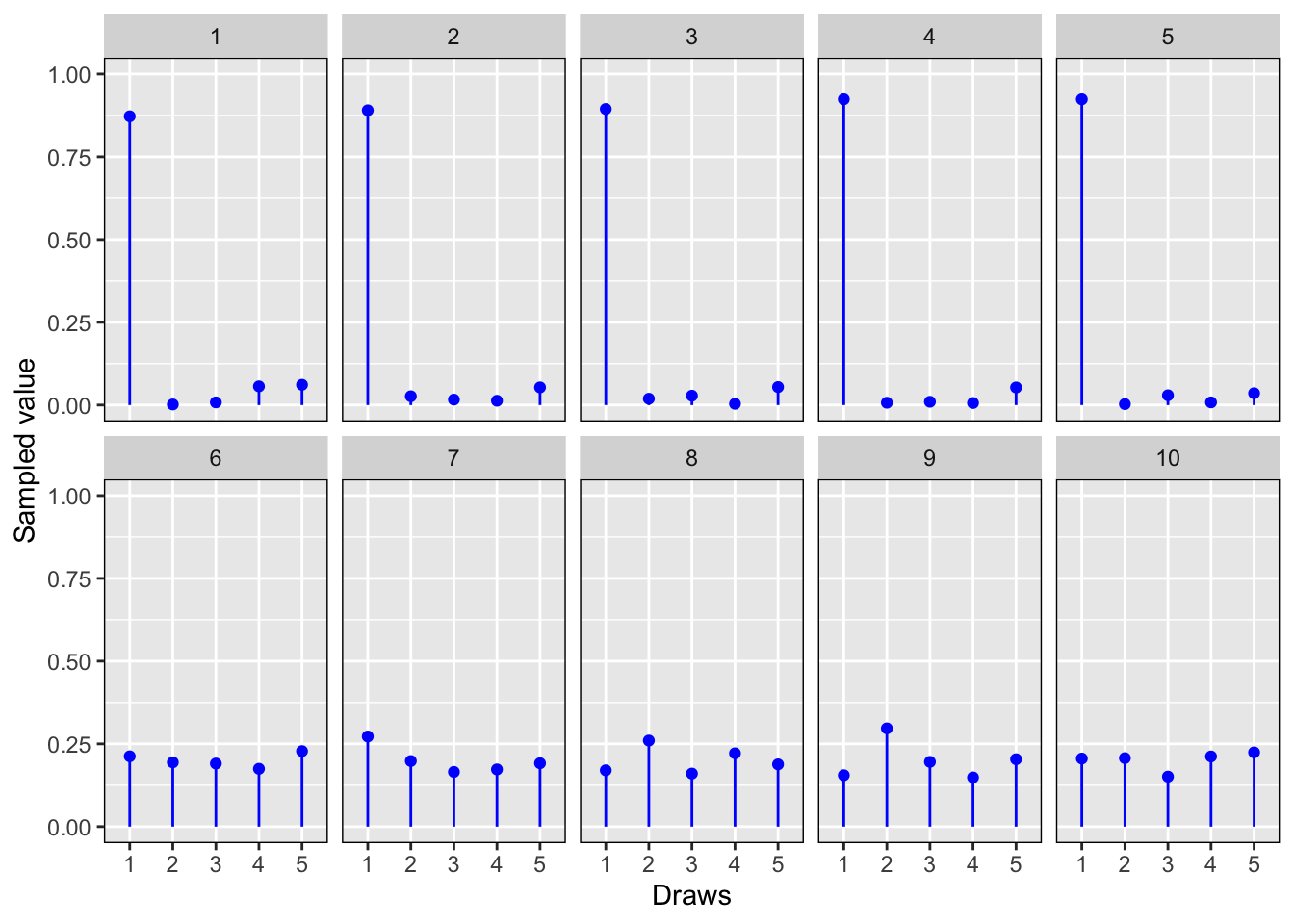
Figure 7.1: Random draws from \(Dir()\) with \(\alpha=10\), \(\rrh_0 = (0.9,0.01,0.01,0.01,0.07)\) and \(\rrh_1=(0.2,0.2,0.2,0.2,0.2)\).
7.3.2 Dirichlet Process Definition
We now formally introduce the Dirichlet process(DP)(Blackwell, MacQueen, et al. 1973).
Let \(\alpha >0\) be the concentration parameter.
Let \(G_0\) be a cumulative distribution function(CDF), referred to as the base measure or base distribution.
Let \(\{B_i\}_{i=1}^{K}\) be a disjoint partition of \(\mathbb{R}\)(note that we focus on \(\mathbb{R}\), but in general we require only a borel sigma algebra).
Then \(G \sim DP(\alpha, G_0)\) is said to follow a DP if for any \(\{B_i\}_{i=1}^{K}\),
\[\begin{align} (G(B_1), \ldots, G(B_K)) \sim Dir(\rrh, \alpha), && \rrh=(G_0(B_1), \ldots, G_0(B_K)) \end{align}\]
7.3.3 DP Visualization
Given \(DP(\alpha, G_0)\), the base distribution \(G_0\) is the expectation of the DP so that for any measurable set \(A \subset \mathbb{R}\), we have \(\mathbb{E}[G(A)] = G_0(A)\).
The concentration parameter \(\alpha\) can be thought of the inverse variance so that greater \(\alpha\) implies lesser variance of DP from \(G_0\).
Draws from \(DP(\alpha, G_0)\) are almost surely discrete(Sethuraman 1994).
Figure 7.2, with base measure \(G_0 = \N(0,1)\), demonstrates the effect of varying \(\alpha\) on the variance of \(G\) drawn from \(DP(\alpha, G_0)\). By observation we see that as \(\alpha \to \infty\) so \(G\) more closely approximates \(G_0\).
The process for drawing \(G\) from \(DP(\alpha, G_0)\) is given in Section 7.4.1.
## Loading required package: startupmsg## Utilities for Start-Up Messages (version 0.9.6)## For more information see ?"startupmsg", NEWS("startupmsg")## Loading required package: sfsmisc## Object Oriented Implementation of Distributions (version 2.9.1)## Attention: Arithmetics on distribution objects are understood as operations on corresponding random variables (r.v.s); see distrARITH().
## Some functions from package 'stats' are intentionally masked ---see distrMASK().
## Note that global options are controlled by distroptions() ---c.f. ?"distroptions".## For more information see ?"distr", NEWS("distr"), as well as
## http://distr.r-forge.r-project.org/
## Package "distrDoc" provides a vignette to this package as well as to several extension packages; try vignette("distr").##
## Attaching package: 'distr'## The following objects are masked from 'package:stats':
##
## df, qqplot, sd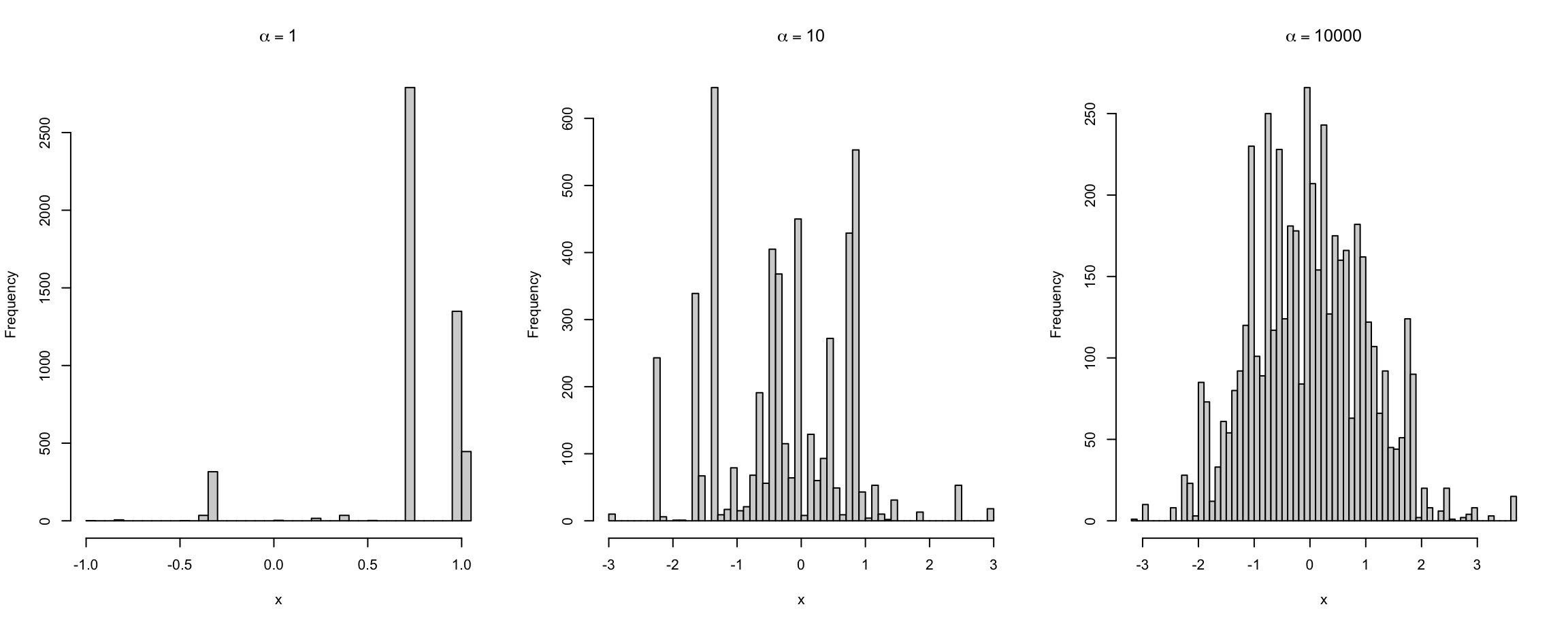
Figure 7.2: Drawing \(G \sim DP(\alpha,G_0)\) with different \(\alpha\).
7.4 Stick Breaking Prior
7.4.1 Sampling with The Stick Break Process
A critical piece of the BNP approach involves the use of a conjugate prior defined on an infinite dimensional parameter space. The default prior is \(DP(\alpha,G_0)\) introduced in the previous section. Although a closed form expression for such a prior exists visualizing the distribution is difficult. The stick breaking process (Sethuraman 1994), provides an algorithm for sampling from \(DP(\alpha, G_0)\) that is both intuitive and easily represented graphically.
The stick breaking process is as follows:
- Draw \(y_1, y_2, \ldots \iid G_0(y)\)
- Draw \(\beta_1, \beta_2, \ldots \iid \mbox{Beta}(1,\alpha)\) and let \(w_k = \beta_k \prod_{i=1}^{k-1}(1-\beta_i)\).
- Let \(G(y) = \sum_{k}w_k \delta_{y_k}\), \(G(y)\) is drawn from \(DP(\alpha, G_0)\).
We begin with a stick of unit length. We draw \(\beta_1\) from \(Beta()\), and break the stick at \(\beta_1\) leaving \((1-\beta_1)\) of the stick. We then draw \(\beta_2\) from \(Beta()\) and break the remaining stick at \(\beta_2(1-\beta_1)\). And this process is repeated \(\textrm{ad infinitum}\). This provides a random sequence \((w_1, w_2,...)\).
Because each interval \(w_i\) on the broken stick is disjoint from the others the basic laws of probability apply to the point masses each portion of the stick represents.
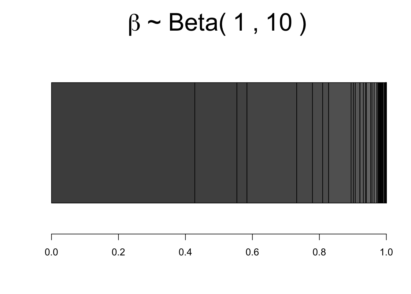
Figure 7.3: Stick breaking process with \(\alpha=10\). Vertical line indicate a \(w_k\)
Figure 7.3 shows the construction of \(w_k\), which covers step 1 and step 2 of the algorithm. Now using the constructed \(w_k\), we can define \(G(y) = \sum_{k}w_k \delta_{y_k}\), where \(\delta_{y_k}\) is a dirac delta function7. Note that in practice we cannot possibly sample infinite \(\beta_k\), so we must instead use some large value \(K\) (truncation value), and sample \(G(y) = \sum_{k=1}^{K}w_k \delta_{y_k}\).
Figure 7.4 illustrates sampling of \(G\) from prior \(DP(\alpha, G_0)\), with \(\alpha = 10\), \(G_0 \sim \N(0,1)\) and \(K = 100\).
library(distr)

# emp_cdf is an object of class "DiscreteDistribution"
cdf_sample <- function(emp_cdf, n=1e3) {
  emp_cdf@r(n)
}

# Dirichlet process to draw a random distribution F from a prior F0
#  alpha determines the similarity with the base measure
#  G_0 is the base measure, a CDF (an object of class "DiscreteDistribution")
dir_process <- function(alpha, G_0, n_atoms=1e3) { # n should be large since it's an approx for +oo
  y_samp <- cdf_sample(G_0,n_atoms)             # step 1: draw from G_0
  betas <- rbeta(n_atoms,1,alpha)               # step 2: draw from beta(1,alpha)
  weights <- c(betas[1], rep(NA,n_atoms-1))                     # step 3: compute 'stick breaking process' into w[i]
  weights[2:n_atoms] <- sapply(2:n_atoms, function(i) betas[i] * prod(1 - betas[1:(i-1)]))

  # return the sampled function F which can be itself be sampled
  # this F is a probability mass function where each s[i] has mass w[i]
  function (size=1e4) {
    sample(y_samp, size, prob=weights, replace=TRUE)
  }
}

# Y is the evidence/data (y1, y2, ..., yn)
dp_posterior <- function(alpha, G_0, Y) {
  n <- length(Y)
  G_n <- DiscreteDistribution(Y) # compute empirical cdf

  G_bar <- n/(n+alpha) * G_n + alpha/(n+alpha) * G_0

  dir_process(alpha+n, G_bar)
}
n_gsamp <- 10        # Number of G to sample
alpha <- c(1,10,1000)  # Concentration parameter
n_atoms <- 1000      # This is the truncation value, K
n_samp <- 1000       # Number of samples to draw from G
g_0 <- function(n) rnorm(n, 0, 1)  # An example base distribution

x_samp = seq(-3,3,len=100)  # x-axis values

par(mfrow=c(1,3))
for(ii in 1:length(alpha)){
  plot(x_samp, pnorm(x_samp), type='l', lwd=2, col="blue", main=bquote(alpha==.(alpha[ii])), xlab="x", ylab="")  # create plot

  for(col_idx in 1:n_gsamp) {
    y <- g_0(n_atoms)
    G_0 <- DiscreteDistribution(y)  # Compute empirical CDF
    G_n <- dir_process(alpha[ii], G_0, n_atoms)  # sample DP
    points(x_samp, ecdf(G_n(n_samp))(x_samp), type='l', col='red')  # plot CDF of sampled G
  }
  legend("topleft",c("True","sampled G"), col=c("blue","red"), lwd=c(2,1), bty = "n")
}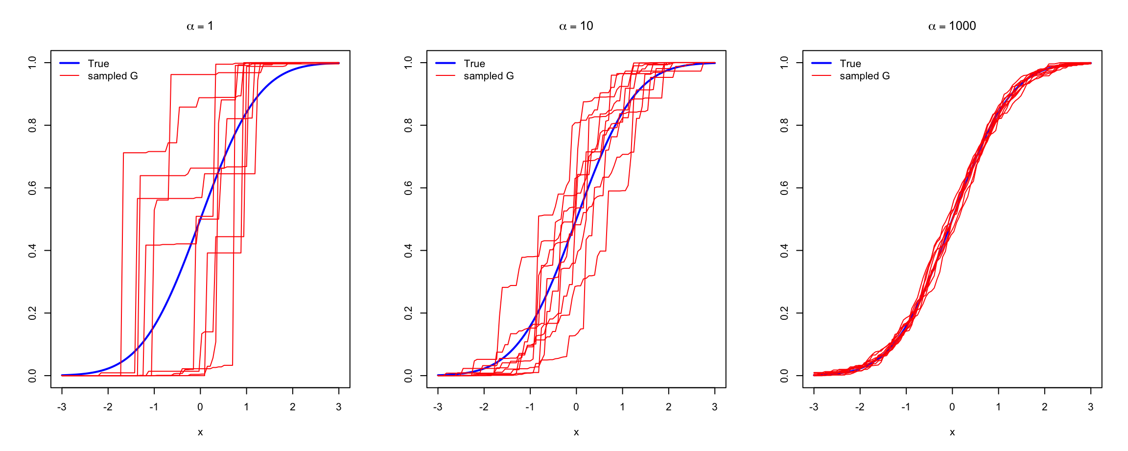
Figure 7.4: An empirical distribution \(G\) sampled from \(DP(\alpha, G_0)\)
7.5 Chinese Restaurant Process
The Chinese Restaurant Process(CRP) (Aldous 1985) is a method for sampling a marginal conditioned on a sample from \(DP(\alpha, G_0)\).
To this point we have constructed the method that allows us to sample \(G \sim DP(\alpha, G_0)\). The next objective is to sample from the induced marginal to get \(Y_1, Y_2, \ldots\) from \(G\). In terms of a model we have: \[ \begin{align*} G &\sim DP(\alpha, G_0) \\ Y_1, Y_2, \ldots Y_n \mid G &\sim G \end{align*} \] The Chinese Restaurant Process (CRP) or infinite Polya urn (Blackwell, MacQueen, et al. 1973) facilitates the exact sampling we now require.
The process is constructed as follows. Let \(Y_1, \ldots, Y_n \sim G\) and let \(G\) have prior \(\mbox{Dir}(\alpha, G_0)\). Then the posterior \(G_n|Y_1, \ldots, Y_n\) is \(\mbox{Dir}(\alpha+n, G_n)\) and, \[\begin{align} G_n = \frac{n}{n+\alpha} \widehat{G_n} + \frac{\alpha}{n+\alpha} G_0 \end{align}\]
Where \(\widehat{G_n}\) denotes the empirical distribution of \(Y_1,\ldots, Y_{n}\).
This theorem implies we can sample \(Y_{n+1}\) from \(G_n\). This stands to reason as the posterior is a DP and we can sample from it as we did before. Remembering De Finetti’s theorem we note that samples drawn from \(G_n\) above are not \(\tx{iid}\) but are exchangeable.
The CRP is as follows:
- Draw \(Y_1 \sim G_0\)
- Draw \(Y_{n+1}\) according to: \[\begin{align} Y_{n+1} \sim \frac{n}{n+\alpha} \widehat{G_n} + \frac{\alpha}{n+\alpha} G_0 = \mbox{DP}(\alpha+n, G_n) \tag{7.2} \end{align}\]
source("../code/bnp/ebook-code.R")
f0 <- function(n) rnorm(n, 1, 1)    # the prior guess (in pdf format)
F0 <- DiscreteDistribution(f0(1000)) # the prior guess (in cdf format)

data <- rnorm(30,3,1)               # the data

# apply Dirichlet process
n_iter  <- 10
xs <- seq(-2,6,len=50)
y_hat <- matrix(nrow=length(xs), ncol=n_iter)
for(i in 1:n_iter) {
  Fpost <- dp_posterior(10, F0, data)
  y_hat[,i] <- ecdf(Fpost())(xs)    # just keeping values of cdf(xs), not the object
}

# plot the black area
plot(xs, pnorm(xs, 1, 1), type="n", ylim=c(-.1,1.1), col="blue", lwd=2, ylab="", xlab="")

# compute & plot 95% credible interval of the posterior
crebible_int <- apply(y_hat, 1, function(row) HPDinterval(as.mcmc(row), prob=0.95))
polygon(c(rev(xs), xs), c(rev(crebible_int[1,]),
                              crebible_int[2,]), col = 'grey90')

# plot the prior cdf
points(xs, pnorm(xs, 1, 1), type="l", col="blue", lwd=2)

# plot mean estimate of the posterior
means <- apply(y_hat, 1, mean)
points(xs, means, type="l", col="red", lwd=2)

# plot true data generator
points(xs, pnorm(xs, 3, 1), type="l", col="darkgreen", lwd=2)
legend("topleft",c("prior","posterior mean", "truth"),
col=c("blue","red","darkgreen"), lwd=2, bty = "n") 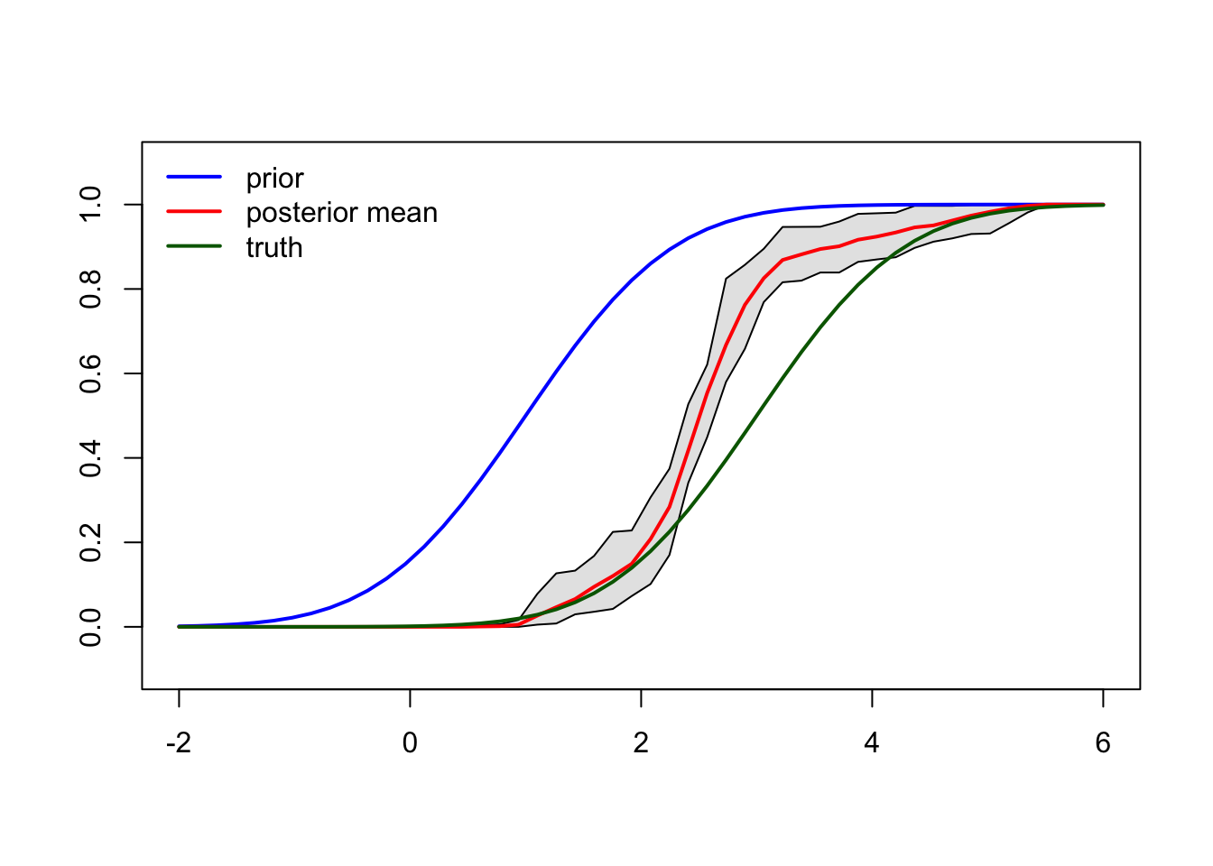
Figure 7.5: CRP posterior prediction and credible interval.
Using (7.2) we can calculate the posterior mean and credible interval around the posterior mean as shown in Figure 7.5.
Why is it called CRP?
The customer \(n+1\) walks into a Chinese8 restaurant, the customer sits at table \(j\) with probability \(\frac{n_j}{n+\alpha-1}\) or sits at new table with probability \(\frac{\alpha}{n+\alpha-1}\).
The \(j\)-th table is associated with dish \(\tilde{Y_j} \sim G_0\).
7.6 Dirichlet Process Mixture Model
To this point we have worked primarily with the CDF of any particular distribution of interest. This is largely due to the fact that DP produces discrete distributions for which the PDF is undefined. We now seek to estimate density function \(f\).
Begin by considering an infinite mixture model used for estimating density, \[\begin{align} f(y) = \sum_{i=1}^{\infty} w_i g(y; \tth_i) \tag{7.3} \end{align}\] In a Bayesian context, we draw \(\tth_i\) from some \(G_0\), and draw \(w_i\) from the stick breaking prior. This infinite mixture is similar to the random distribution \(G \sim \mbox{DP}(\alpha, G_0)\) which had the form \(G = \sum_{i=1}^{\infty} w_i \delta_{\tth_i}\); only the dirac delta is replaced by kernel function \(g(\cdot)\) with smooth densities.
The Dirichlet process mixture model (DPMM) (Radford M. Neal 2000) is defined as: \[\begin{align} G &\sim \mbox{DP}\{G_0, \alpha\} \nonumber \\ \tth_1, \ldots, \tth_n &\sim G \tag{7.4} \\ \YY_i \mid \tth_i &\ind f(\yy \mid \tth_i) \nonumber \end{align}\]
Note that since \(G\) is discrete, and the \(\tth_i\)’s are sampled from \(G\), the \(\tth_i\) will have ties. Therefore, the number of unique \(\tth_i\) can be thought of as defining clusters. This implicitly defines a prior on the number of distinct \(\tth_i\)’s.
7.6.1 DPMM Inference
Here we describe inference with the model (7.4).
In practice, the user might impose a prior on \(\alpha\) and the parameters of \(G_0\)(Escobar and West 1995). Let \(\TTh = (\tth_1, \ldots, \tth_n)\) and let \(\TTh_{-i}\) be \(\TTh\) with \(\tth_i\) removed. Based on the CRP sampler (Radford M. Neal 2000), the posterior distribution for \(\tth_i\) conditional on the other model parameters is: \[\begin{align} p(\tth_i \mid \TTh_{-i}, \YY, \alpha, G_0) &= \sum_{j \neq i} q_j \delta_{\theta_j} + r \cdot p(\tth_i \mid \alpha, G_0, \YY) \tag{7.5}\\ q_j &\propto \frac{g(\yy_i; \tth_j)}{\alpha+ n - 1} \nonumber \\ r &\propto \frac{\alpha}{\alpha + n -1} \int g(\yy_i; \tth) \, dG_0(\tth) \nonumber \end{align}\]
Recall from earlier CRP discussion that the \(\tth_i\) are exchangeable which causes samples from (7.5) to be invariant over the permutations on \(i\). Given the posterior MCMC algorithms are used to do inference. The most notable inference algorithm for DPMM is the one introduced in (Radford M. Neal 2000) for DPMM with conjugate prior pair which provides a closed form PDF for (7.5).
In the absence of a closed form distribution, as in the non-conjugate case, (7.5) still holds but additional steps are required for inference. The reader may refer to “Algorithm 8” in (Radford M. Neal 2000) for details.
7.7 Practical Application
This section provides a brief introduction to the direchletprocess package in R.
As with many statistics and machine learning packages the dirichletprocess package includes a number of
datasets that allow you to experiment with and learn the capabilities of the package.
The authors of dirichletprocess package also provide a number of tutorials online.
The following sections provide some repackaged high-lights from the tutorials
to facilitate the user with an intuition for practical BNP methods. While the examples provided are not necessarily
difficult or rigorous, paying attention to the details of execution will provide an added dimension of insight
into the material previously covered.
7.7.1 Practical Example Requirements
The following examples can be run in any number of different environments. Rstudio is an often used tool that enables browsing the stack, and referenced memory locations in the R kernel. The following assumes a bare bones R installation, and is intended to be run from the R console command line. Code snippets may be cut and past into the console, or an R script as desired.
To run the following examples you are required to have:
an R installation \(\geq\) 3.6.3 (lesser versions may work but are untested)
the following packages installed:
- dirichletprocess
- ggplot2
- tidyr
To install required packages, bring up an R console and issue the following commands:
install.packages("dirichletprocess")
install.packages("ggplot2")
install.packages("tidyr")
7.7.2 Simple Density Estimation Using DPMM
We begin with we will take a look at some data for old faithful (the much beloved geyser in Yellowstone National Park) and run through the steps required to build a model for it.
library(dirichletprocess)
library(ggplot2)head(faithful)## eruptions waiting
## 1 3.600 79
## 2 1.800 54
## 3 3.333 74
## 4 2.283 62
## 5 4.533 85
## 6 2.883 55ggplot(faithful, aes(x=waiting)) + geom_histogram(binwidth = 1)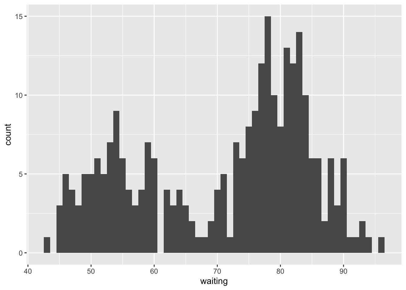
Figure 7.6: old faithful data table and histogram
Looking at the data table and histogram in Figures 7.6 we see a possibly bi-modal distribution, where longer wait times probably produce geyser eruptions of longer duration. We note that while it may be true that the time to wait and duration of previously occurring eruptions may impact the same for the presently occurring eruption - so that the sequence is not necessarily independent - rearranging the order of the data set does not impact its statistics - so the sequence is exchangeable; thus the sequence may be a good candidate for BNP modeling.
From a parametric perspective, we could model this data using a mixture of two Gaussians. This may well work for this data set, however there are many cases where the choice may not be so obvious - and it may be that our naive observation of the data over-looks some subtle nuance. With BNP we can model the data without making arbitrary, possibly unfounded decisions, about its modes. Instead we let the model learn the necessary number of parameters from the data by setting up a DPMM to estimate the unknown density \(f(y)\) as follows: \[\begin{align} G &\sim \text{DP}(\alpha, G_0) \nonumber \\ f(y) &= \int g(y \mid \tth) p(\tth \mid G) \mathrm{d} \theta \tag{7.6}\\ \end{align}\]
With \(g(y \mid \theta)\) as a mixture density, \(G\) sampled from Dirichlet process prior with \(G_0\) base distribution, and concentration parameter \(\alpha\).
Using the dirichletprocess package we can easily define \(g(y \mid \tth)\) as a Gaussian kernel with \(\tth = (\mu, \sigma^2)\):
\[
\begin{align}
g(y \mid \theta) = N(y \mid \mu,\sigma^2) \\
\end{align}
\]
Recall from section 7.6.1 we need to place priors on the parameters of \(G_0\). Using \(\gamma=(\mu_0, \kappa_0, \alpha_0, \beta_0)\) we define:
\[\begin{align}
G_0(\tth \mid \gamma) = \N \left( \mu \mid \mu_0, \frac{\sigma^2}{\kappa_0} \right) \mbox{Inv-Gamma}\left( \sigma^2 \mid \alpha_0, \beta_0\right)
\end{align}\]
# Normalize the data set
faithfulTrans <- (faithful$waiting - mean(faithful$waiting))/sd(faithful$waiting)
# Create a DP  with the Gaussian as its base
dp <- DirichletProcessGaussian(faithfulTrans)
# Check process details
dp
## Dirichlet process object run for 0 iterations.
##
## Mixing distribution normal
## Base measure parameters 0, 1, 1, 1
## Alpha Prior parameters 2, 4
## Conjugacy conjugate
## Sample size 272
## Now we perform a fit.
# Perform fit
dp <- Fit(dp, 1000, progressBar = FALSE)
Tht fitting function calculates the conjugate posterior: \[\begin{align} p(\tth \mid y, \gamma) &= \N\left( \mu \mid \mu_n, \frac{\sigma^2}{\kappa_0 + n}\right) \mbox{Inv-Gamma}\left( \sigma^2 \mid \alpha_n, \beta_n \right) \\ \mu_n &= \frac{\kappa_0\mu_0 + n \bar{y}}{\kappa_0 + n} \\ \alpha_n &= \alpha_0 + \frac{n}{2} \\ \beta_n &= \beta_0 + \frac{1}{2} \sum_{i=1}^{n}(y_i - \bar{y})^2 + \frac{\kappa_0n(\bar{y}-\mu_0)}{2(\kappa_0 + n)} \end{align}\]
plot(dp)## Warning: The `<scale>` argument of `guides()` cannot be `FALSE`. Use "none" instead as
## of ggplot2 3.3.4.
## ℹ The deprecated feature was likely used in the dirichletprocess package.
## Please report the issue at
## <https://github.com/dm13450/dirichletprocess/issues>.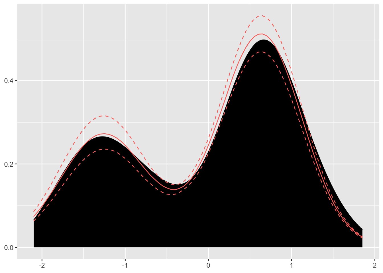
Figure 3.6: Plot of posterior mean and credible interval
Looking inside the Dirichlet process object, we see the model was fit as follows:
# Looking under the hood of the Dirichlet Process object
data.frame(Weights=dp$weights,
                  mu=c(dp$clusterParameters[[1]]),
                  sigma=c(dp$clusterParameters[[2]]))
## Weights mu sigma
## 1 0.330882353 -1.27297501 0.5111741
## 2 0.599264706 0.64272546 0.4838292
## 3 0.018382353 -0.28109140 1.0363500
## 4 0.029411765 -0.06234216 0.7502674
## 5 0.011029412 -0.54488372 0.6752711
## 6 0.003676471 0.59582202 1.5368170
## 7 0.003676471 -1.23421616 0.6992793
## 8 0.003676471 -3.30131353 2.9330700So with only a few lines of code the dirichletprocess package has provided a DPMM, a fit for the data, and credible intervals.
7.7.3 Custom Mixture Models
BNP methods provide a significant degree of flexibility in terms of model construction. DPMM as described in Equations (7.3) and (7.4) demonstrate this flexibility by leaving choices with regards to the specific form of its various elements. But as section 7.6.1 describes, convenient choices involving the use of conjugate priors simplify the math by making available closed form expressions from which to draw.
In this section we take advantage of this flexibility by constructing a mixture model based on \(f\) as a mixture of \(Exp(\theta)\) and its conjugate prior the \(\mbox{Gamma}()\).
Following the form of Equations (7.3) and (7.4) closely, we seek to develop a generative model specified as follows:
\[\begin{align} \pi(\alpha) &= \mbox{Gamma}(a_0, b_0) \\ G_0 &= \mbox{Gamma}(a_1, b_1)\\ G &\sim DP\{\alpha, G_0\} \tag{7.7} \\ \theta_i &\sim G \\ Y_i \mid \theta_i &\sim \sum_{1}^{\infty} w_i \theta_i \exp^{-\theta_i y_i}\\ \end{align}\]
The posterior from (7.7) is: \[\begin{align} \theta \mid y_1,...,y_n &\sim \mbox{Gamma}(a_1 + n, b_1 + \sum_{i}^{n} y_i) \tag{7.8}\\ \end{align}\]
We begin by creating a mixing distribution object to over-ride the default mixing distribution linked when the dirichlet process object is instantiated. The “exp” tag label is affixed to the other functions that make up the model so that they can be linked to the model.
The priorParameters \((0.1, 0.1)\) are passed in for \((a_1, b_1)\) and the conjugate label identifies the model as a conjugate pair:
# Mixing Distribution
library(dirichletprocess)
library(ggplot2)
a1 = 0.1
b1 = 0.1
expMd <- MixingDistribution(distribution = "exp", priorParameters = c(a1,b1), conjugate = "conjugate")
The likelihood of our model data is described as an exponential distribution given \(\theta\):
# Likelihood
Likelihood.exp <- function(mdobj, y, theta){
  as.numeric(dexp(y, theta[[1]]))
}
The prior draw method is defined as \(\mbox{Gamma}()\) with the current prior parameters:
# Prior Draw
PriorDraw.exp <- function(mdobj, n){
  draws <- rgamma(n, mdobj$priorParameters[1], mdobj$priorParameters[2])
  theta <- list(array(draws, dim=c(1,1,n)))
  return(theta)
}
We implement the posterior draw as in Equation (7.8), drawing \(\theta\) conditional on the data from the posterior using the \(\mbox{Gamma}()\):
# Prior Draw
PosteriorDraw.exp <- function(mdobj, y, n=1){
  priorParameters <- mdobj$priorParameters
  theta <- rgamma(n, priorParameters[1] + length(y), priorParameters[2] + sum(y))
  return(list(array(theta, dim=c(1,1,n))))
}
Using: \[\begin{align} p(y) &= \int p(y \mid \theta) p(\theta) \mathrm{d} \theta \tag{7.9} \\ \end{align}\]
The predictive function is an estimate of the marginal \(p(y)\) in (7.9):
# Predictive Function
Predictive.exp <- function(mdobj, y){
  priorParameters <- mdobj$priorParameters
  pred <- numeric(length(y))
  for(i in seq_along(y)){
    alphaPost <- priorParameters[1] + length(y[i])
    betaPost <- priorParameters[2] + sum(y[i])
    pred[i] <- (gamma(alphaPost)/gamma(priorParameters[1])) * ((priorParameters[2] ^priorParameters[1])/(betaPost^alphaPost))
  }
  return(pred)
}
We now create the Dirichlet process, over-riding the default mixing function with expMd, and fit some test data:
# Predictive Function
yTest <- c(rexp(100, 0.1), rexp(100, 20))
dp <- DirichletProcessCreate(yTest, expMd)
dp <- Initialise(dp)
dp <- Fit(dp, 1000, progressBar = FALSE)
data.frame(Weight=dp$weights, Theta=unlist(c(dp$clusterParameters)))
## Weight Theta
## 1 0.36 19.63250901
## 2 0.50 0.08551698
## 3 0.14 12.61755754We see that the data has been fit relatively well. We leave it to the reader to experiment.
7.8 Resources
As often it is the case in mathematics, so it is with BNP, reading and understanding multiple treatments of the same subject matter leads to understanding.
We encourage the reader to take advantage of the opportunity the internet presents in this regard.
We thank, endorse, and acknowledge the following (re)sources:
- Names worth a Google
- Michael I. Jordan
- Tamara Broderick
- Yee Whye Teh
- Peter Orbanz
- Larry A. Wasserman
- Gordon J. Ross, Dean Markwick, Kees Mulder, Giovanni Sighinolfi, Dean Markwick (the dirichletprocess team)
- General introduction to nonparametric methods
- Inference with DPMM
- Landmark paper on Gibb’s type MCMC sampling for DPMM (Radford M. Neal 2000)
- Bayesian Inference with DPMM (Escobar and West 1995)
- Use of DPMM targeted to machine learning audience (Rasmussen 2000)
- Prior Construction (Theory heavy)
- Mathematically rigourous treatment of prior construction (Eldredge 2016)
- Yee Whye Teh’s note
- Online Video Lectures
- R packages
- dirichletprocess used in examples
- MCMCpack used for sampling dirichlet distribution
- distr used for wrapping empirical CDF’s computation
- ggplot2 used for visualization