Univariate Distributions as xDensity Objects

Martin Lysy, Jonathan Ramkissoon

2019-11-01

Introduction

The GaussCop package proposes a simple, unified framework to provide the basic d/p/q/r functions for arbitrary continuous one-dimensional distributions. This can be useful for working with various Copula models (including the Gaussian Copula in the example below).

xDensity Objects

Let \(X\) denote an unbounded, continuous random variable with PDF \(X \sim f(x)\). An xDensity object essentially consists of the following elements:

• PDF values on an evenly-spaced grid.
• The mean and standard deviation of a Normal distribution to be used outside the grid.

Based on this representation, the d/p/q/r functions are implemented as follows:

• PDF (d): Step function inside the grid, Normal outside the grid.
• CDF (p): Piecewise linear inside the grid, Normal outside the grid.
• Inverse-CDF (q): Exact numerical inversion of the CDF.
• Sampling (r): Inverse-CDF method. That is, if \(F(x)\) is a CDF and \(U \sim \mathrm{Unif}(0,1)\), then \(X = F^{-1}(U)\) has CDF \(F(x)\).

Basic Usage

xDensity objects can be constructed either from iid samples \(X_{1},\ldots,X_{n} \stackrel{\mathrm{iid}}{\sim}f(x)\) or from a functional representation of \(f(x)\) itself. For example, consider the following xDensity representation based on a random sample from the log-Exponential distribution, \[ \log(X) \sim \mathrm{Expo}(1) \qquad \iff \qquad f(x) = \exp(-e^x + x). \]

require(GaussCop) # load package

## Loading required package: GaussCop

# simulate data
nsamples <- 1e5
X <- log(rexp(nsamples)) # iid samples from the log-Exponential

xDens <- kernelXD(X) # basic xDensity constructor
names(xDens)

## [1] "ndens" "xrng"  "ypdf"  "ylpdf" "ycdf"  "mean"  "sd"

The elements of xDens are:

• ndens, xrng: a compact representation of the \(x\)-value grid, i.e., the number of grid points and the range of the grid.
• ypdf, ylpdf, ycdf: the PDF, log-PDF, and CDF evaluated at the ndens grid points. While the latter two elements can be reconstructed from the first, they are stored here in order to speed up subsequent calculations.
• mean, sd: The mean and variance of the Normal distribution used outside the range of the grid. By default, these values are chosen by matching the Normal PDF to the ypdf values at then endpoints of the grid; details of the calculation can be found in the Appendix .

The d/p/q/r functions for xDensity objects are invoked by e.g.:

dXD(x, xDens = xDens, log = TRUE) # log-PDF
pXD(x, xDens = xDens, lower.tail = FALSE) # survival function (1-CDF)
qXD(p = .5, xDens = xDens) # median
rXD(n, xDens = xDens) # random sample

To assess the quality of the xDensity approximation to the log-Exponential distribution \(\log(X) \sim \mathrm{Expo}(1)\), consider the following checks:

1. That the histogram of rXD() sample matches dXD() and the true PDF (recall that rXD() calls qXD() on stats::runif()).
2. That pXD() matches the true CDF.

These graphical checks are implemented by the function xdens_test (R code in Appendix) as illustrated below:

# check that xDensity d/p/q/r functions match the true distribution,
# by plotting true PDF/CDF vs xDensity representation.

dlexp <- function(x) exp(-exp(x) + x) # true PDF
plexp <- function(x) pexp(exp(x)) # true CDF

xdens_test(xDens, # xDensity approximation 
           dtrue = dlexp, # true PDF 
           ptrue = plexp, # true CDF
           dname = expression(log(X)%~%"Expo"*(1)), # name of true distribution (for legend)
           dlpos = "topleft", plpos = "topleft") # legend position for pdf/cdf plot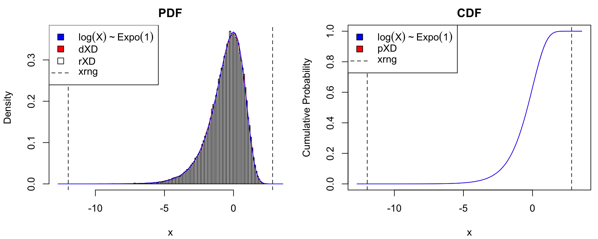

Graphical assessment of xDensity approximation to the log-Exponential distribution.

Constructors for xDensity Objects

The GaussCop package currently implements three methods of constructing xDensity objects. Two take as input a random sample \(X_{1},\ldots,X_{n} \sim f(x)\). The third is based on a functional approximation \(\hat f(x)\), e.g., as resulting from a parametric model \(\hat f(x) = f(x \mid \hat {\boldsymbol{\theta}})\), where \(\hat{\boldsymbol{\theta}}\) is the parameter MLE.

Kernel Density Estimation

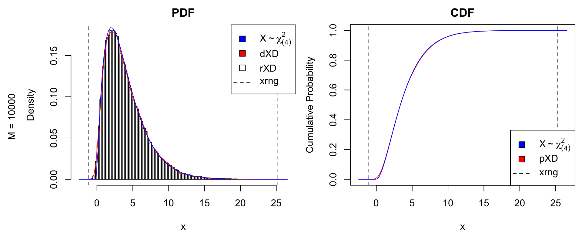
The kernelXD() function uses the stats::density() function to fit a Gaussian kernel to a random sample from \(f(x)\). It is the most flexible constructor; however, it also requires the most datapoints for stable estimation. Below is a comparison with \(M\) iid samples from a \(\chi^2_{(4)}\) distribution, using \(M = 1000\) and \(M = 10000\) data points.

# true distribution: chi^2_(4)
df_true <- 4
dtrue <- function(x) dchisq(x, df = df_true)
ptrue <- function(x) pchisq(x, df = df_true)
rtrue <- function(n) rchisq(n, df = df_true)
dname <- paste0("X%~%chi[(",df_true,")]^2")

# simulate data
nsamples <- 1e3
X <- rtrue(nsamples)
xDens <- kernelXD(X) # xDensity constructor

par(oma = c(0,2,0,0)) # put sample size in outer margin
xdens_test(xDens, dtrue = dtrue, ptrue = ptrue,
           dname = dname,
           dlpos = "topright", plpos = "bottomright")
mtext(text = paste0("M = ", nsamples),
      side = 2, line = .5, outer = TRUE)

# increase sample size
nsamples <- 1e4
X <- rtrue(nsamples)
xDens <- kernelXD(X)
xdens_test(xDens, dtrue = dtrue, ptrue = ptrue,
           dname = dname,
           dlpos = "topright", plpos = "bottomright")
mtext(text = paste0("M = ", nsamples),
      side = 2, line = .5, outer = TRUE)
par(oma = c(0,0,0,0)) # remove outer margin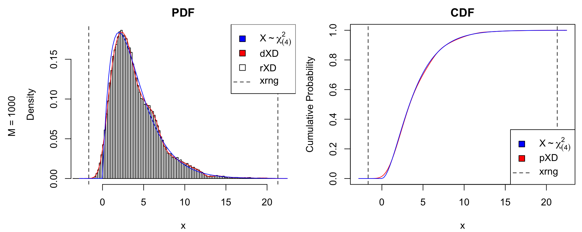

Impact of sample size on quality of kernelXD() approximation.

Gram-Charlier Expansion

The gc4XD() constructor implements a moment-based density approximation, which works best for unimodal distributions that are not too far from normal. The estimator proceeds in two steps:

1. The data \(X_{1},\ldots,X_{n} \stackrel{\mathrm{iid}}{\sim}f(x)\) are first normalized by applying a Box-Cox transformation to each observation \(X_i\), \[Z_i = \mathrm{BoxCox}(X_i \,|\, \hat \alpha, \hat \lambda), \qquad \mathrm{BoxCox}(x \,|\, \alpha, \lambda) = \begin{cases} \frac{((x + \alpha)^\lambda - 1)}{(\lambda C^{\lambda-1})} & \lambda \neq 0 \\ C \log(x + \alpha) & \lambda = 0, \end{cases} \] where \((\hat \alpha, \hat \lambda)\) are obtained by maximum likelihood.
2. The transformed data \(Z_{1},\ldots,Z_{n}\) are then fit with a 4th order Gram-Charlier expansion (e.g., Draper and Tierney 1972). That is, let \(\hat \mu\), \(\hat \sigma\), \(\hat \kappa_3\), and \(\hat \kappa_4\) denote the sample-based estimates of the first four cumulants of \(Z = \mathrm{BoxCox}(X \,|\, \hat \alpha, \hat \lambda)\). The 4th order Gram-Charlier approximation to the true PDF \(f(z)\) is \[ \hat f(z) = \frac{1}{\sqrt{2\pi}\hat \sigma} \exp\left[-\frac{(z-\hat \mu)^2}{2\hat\sigma^2}\right] \times \left[1 + \frac{\hat \kappa_3}{3!\hat \sigma^3} H_3\left(\frac{z-\hat\mu}{\hat\sigma}\right) + \frac{\hat \kappa_4}{4!\hat\sigma^4} H_4\left(\frac{z-\hat\mu}{\hat\sigma}\right)\right], \] where \(H_3(z) = z^3 - 3z\) and \(H_4(z) = z^4 - 6z^2 + 3\) are the 3rd and 4th Hermite polynomials. The approximation \(\hat f(z)\) is not guaranteed to be positive, but generally is for reasonably unimodal distributions, in which case \(\hat f(z)\) is a (normalized) PDF with mean, variance, skewness and kurtosis exactly matching those of the transformed data \(Z_{1},\ldots,Z_{n}\).

The gc4XD() constructor estimates the PDF of the data \(X_{1},\ldots,X_{n}\) on the original scale by inverting steps 1 and 2 above. The example below illustrates the quality of the approximation for \(M = 1000\) observations of \(X \sim \chi^2_{(4)}\).

nsamples <- 1e3
X <- rtrue(nsamples)
xDens <- gc4XD(X) # xDensity constructor
xdens_test(xDens, dtrue = dtrue, ptrue = ptrue,
           dname = dname,
           dlpos = "topright", plpos = "bottomright")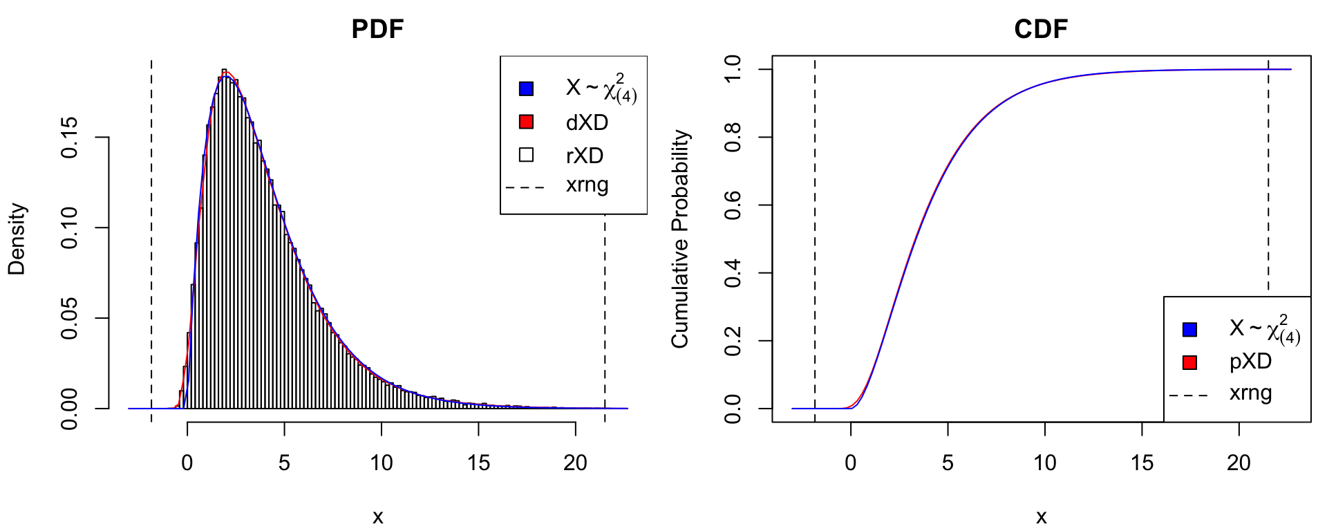

gc4XD() approximation with \(M = 1000\) samples.

Known Density Values

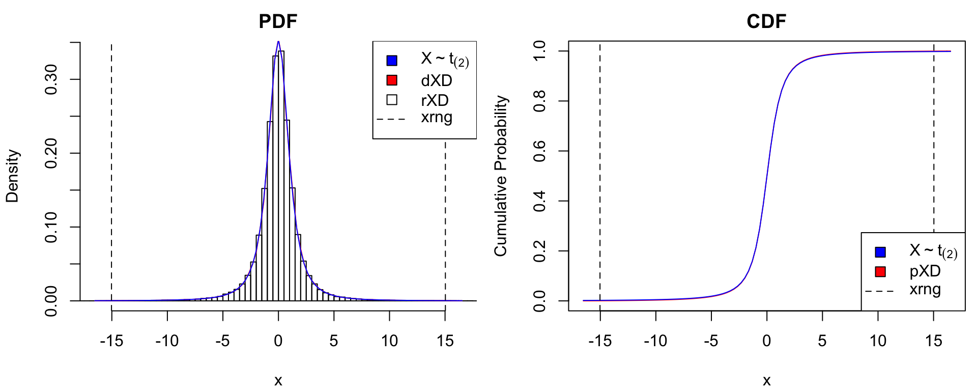
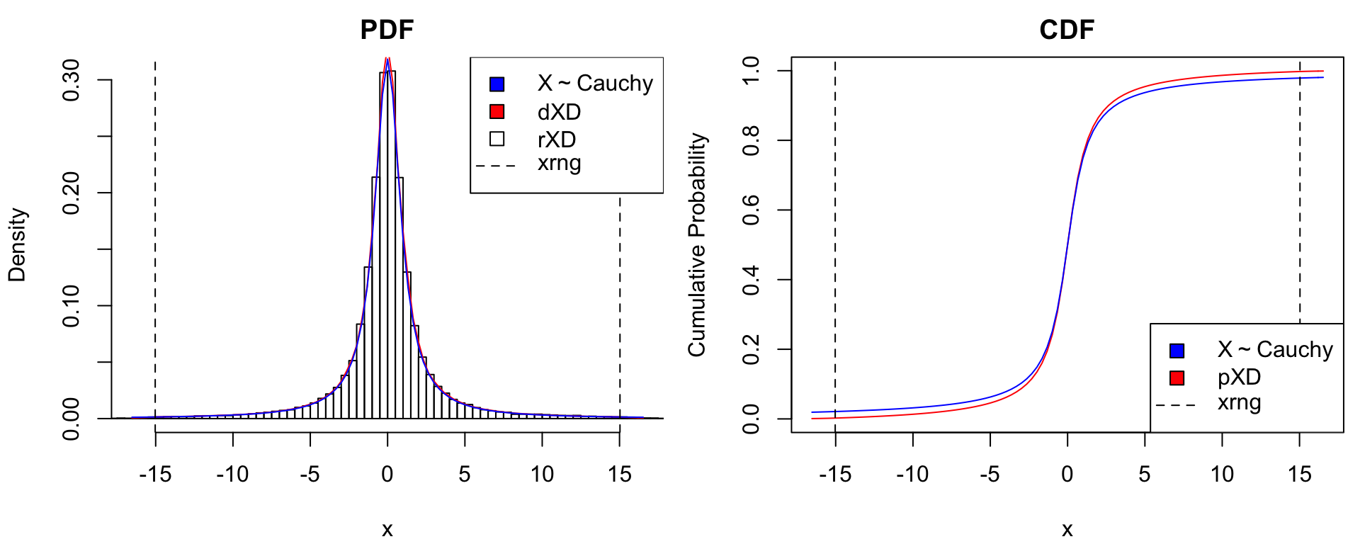
The matrixXD() constructor is used to convert functional density representations into the standardized xDensity format. Its input is a 2-column matrix with equally-spaced \(x\)-grid values in the first column and corresponding density values in the second. Below is an illustration using the Student-\(t\) distributions \(X \sim t_{(2)}\) and \(X \sim t_{(1)}\) (i.e., Cauchy) distributions. We can see that for extremely heavy-tailed distributions such as Cauchy, the normal approximation used by xDensity clearly undercuts tail probabilities.

# true distribution: t(2)
dtrue <- list(t2 = function(x) dt(x, df = 2),
              Cauchy = function(x) dt(x, df = 1))
ptrue <- list(t2 = function(x) pt(x, df = 2),
              Cauchy = function(x) pt(x, df = 1))
dname <- expression(X%~%t[(2)], X%~%"Cauchy")

# matrix density representation
xgrid <- seq(from=-15, to=15, len = 500) # grid
for(ii in 1:2) {
  ypdf <- dtrue[[ii]](xgrid) # true density
  xDens <- matrixXD(cbind(X = xgrid, Y = ypdf)) # xDensity constructor
  xdens_test(xDens, dtrue = dtrue[[ii]], ptrue = ptrue[[ii]],
             dname = dname[ii],
             dlpos = "topright", plpos = "bottomright")
}

matrixXD() approximation for \(t_{(\nu)}\) distributions with \(\nu = 1,2\).

Application: The Gaussian Copula Distribution

Consider a \(d\)-dimensional random variable \({\boldsymbol{X}}= (X_{1},\ldots,X_{d})\) with unknown PDF \({\boldsymbol{X}}\sim f({\boldsymbol{x}})\). A popular approach to statistical dependence modeling is to do so upon transforming \({\boldsymbol{X}}\) to having univariate margins. That is, if \(F_i(x_i)\) is the CDF of \(X_i\), then \[ U_i = F_i^{-1}(X_i) \sim \mathrm{Unif}(0,1), \] such that the joint PDF of \({\boldsymbol{X}}\) can be written as \[ f({\boldsymbol{x}}) = c({\boldsymbol{u}}) \times\prod_{i=1}^n f_i(x_i), \qquad u_i = F_i(x_i). \] Thus, \(c({\boldsymbol{u}})\) is the joint PDF of marginally Uniform random variables, \(U_i \sim \mathrm{Unif}(0,1)\), and is known as a Copula distribution. Numerous R packages provide various for fitting and sampling from Copula distributions, e.g., copula (Hofert et al. 2017), VineCopula (Schepsmeier et al. 2017), and many others listed in the Distributions Task View. The xDensity methods for modeling the marginal distributions \(f_i(x_i)\) can easily be combined with the Copula dependence models \(c({\boldsymbol{u}})\) provided by these packages. GaussCop provides a simple and specific interface to the so-called Gaussian Copula distribution, which approximates the true \(c({\boldsymbol{u}})\) as follows:

1. Let \(\varphi(z)\) and \(\Phi(z)\) denote the PDF and CDF of the standard normal \({\mathcal N}(0,1)\). Now, consider the change-of-variables \(Z_i = \Phi^{-1}(U_i)\), for which the joint PDF of \({\boldsymbol{Z}}= (Z_{1},\ldots,Z_{n})\) is \[ g({\boldsymbol{z}}) = c({\boldsymbol{u}}) \times \prod_{i=1}^n \varphi(z_i), \qquad u_i = \Phi(z_i). \]
2. Since marginally \(Z_i \sim {\mathcal N}(0,1)\), the Gaussian Copula approximates the true distirbution \(g({\boldsymbol{z}})\) by the best-matching multivariate normal, in the sense of minimizing the Kullback-Leibler divergence, \[ \hat g({\boldsymbol{z}}) = \mathrm{argmin}_{{\boldsymbol{R}}} \int \log \left[\frac{g({\boldsymbol{z}})}{\varphi({\boldsymbol{z}}\mid {\boldsymbol{R}})}\right] \cdot g({\boldsymbol{z}}) \,\mathrm{d}{\boldsymbol{z}}, \] where \(\varphi({\boldsymbol{z}}\mid {\boldsymbol{R}})\) is the joint PDF of a multivariate normal \({\mathcal N}(0, {\boldsymbol{R}})\) with correlation matrix \({\boldsymbol{R}}_{ii} = 1\).

To evaluate the accuracy of the Gaussian Copula appromation, consider applying it to the \(p(p+1)/2\)-dimensional Cholesky decomposition of a “unit” \(p\times p\) Wishart distribution, \[ {\boldsymbol{X}}_{p\times p} \sim \mathrm{Wishart}({\boldsymbol{I}}, p). \] That is, \({\boldsymbol{X}}= {\boldsymbol{Z}}'{\boldsymbol{Z}}\) and \({\boldsymbol{Z}}\) is a \(p\times p\) matrix of iid \({\mathcal N}(0,1)\).

By construction, the Gaussian Copula perfectly captures the marginal distributions of \(\mathrm{chol}({\boldsymbol{X}})\). Therefore, consider the error on the marginal distributions of the eigenvalues of \({\boldsymbol{X}}\), induced by approximating the copula dependence between the Cholesky variables as multivariate normal. In the example below with \(p = 4\), the error appears to be relatively small:

# simulate data from unit Wishart distribution
p <- 4 # size of matrix
nsamples <- 1e4
X <- replicate(nsamples, crossprod(matrix(rnorm(p^2),p,p)))

# Cholesky decomposition
Xchol <- apply(X, 3, function(V) chol(V)[upper.tri(V,diag = TRUE)]) 
Xchol <- t(Xchol)

# fit Gaussian Copula approximation
gCop <- gcopFit(X = Xchol, # iid sample from multivariate distribution
                fitXD = "kernel") # xDensity approximation to each margin

# Compare approximation to true distribution of eigenvalues of X

# extract sorted eigenvalues of a positive definite matrix
eig_val <- function(V) {
  sort(eigen(V, symmetric = TRUE)$values, decreasing = TRUE)
}

Xeig <- t(apply(X, 3, eig_val)) # true distribution
Xeig2 <- rgcop(nsamples, gCop = gCop) # Gaussian Copula approximation
Xeig2 <- t(apply(Xeig2, 1, function(U) {
  # recover full matrix
  V <- matrix(0,p,p)
  V[upper.tri(V,diag=TRUE)] <- U
  V <- crossprod(V)
  eig_val(V)
}))

# plot true and approximate eigenvalue distributions
main <- parse(text = paste0("lambda[", 1:p, "]"))
par(mfrow = c(1,p), mar = c(2.5,2.5,2,.1)+.1, oma = c(0,2,0,0))
for(ii in 1:p) {
  dtrue <- density(Xeig[,ii])
  dapprox <- density(Xeig2[,ii])
  xlim <- range(dtrue$x, dapprox$x)
  ylim <- range(dtrue$y, dapprox$y)
  plot(dtrue$x, dtrue$y, type = "l", xlim = xlim, ylim = ylim,
       main = main[ii], xlab = "", ylab = "", col = "blue")
  lines(dapprox$x, dapprox$y, col = "red")
}
mtext(text = "Density",
      side = 2, line = .5, outer = TRUE)
legend("topright", legend = c("True PDF", "gCop Approx."),
       fill = c("blue", "red"))
par(oma = c(0,0,0,0)) # remove outer margin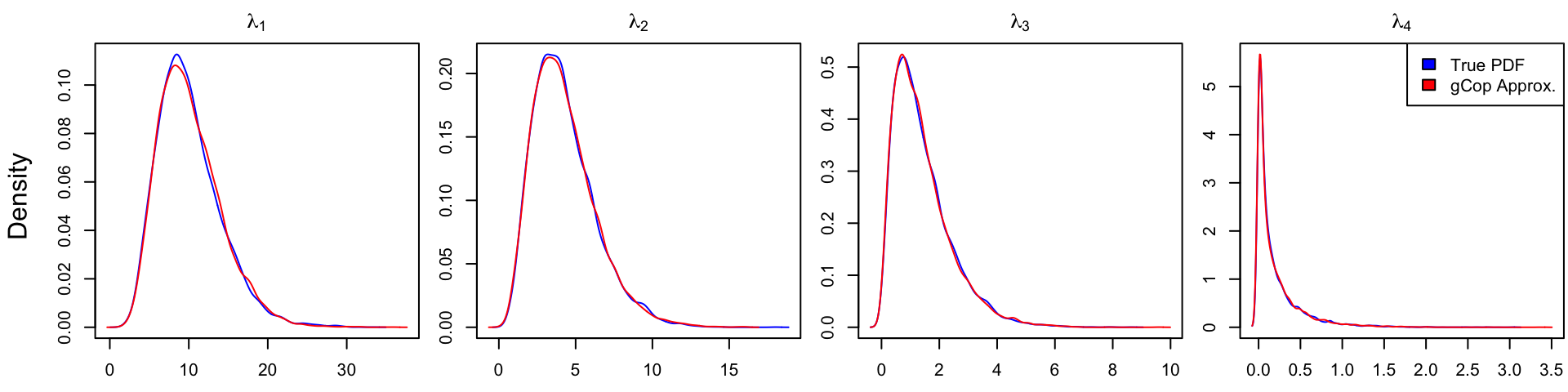

Gaussian Copula approximation to the eigenvalues of \({\boldsymbol{X}}\sim \mathrm{Wishart}({\boldsymbol{I}}, 4)\), as fitted to \(\mathrm{chol}({\boldsymbol{X}})\).

Appendix A: Endpoint Matching

We wish to find the parameters \((\mu, \sigma)\) of a normal distribution whose PDF passes through the points \((x_i, y_i)\), \(i = 1,2\). Thus we wish to find \((\mu, \sigma)\) satisfying \[ \log y_i = -\frac 1 2 \left[\frac{(x_i - \mu)^2}{\sigma^2} + \log \sigma^2 + \log 2\pi \right], \qquad i = 1,2. \] Subtracting one equation from the other, we obtain \[ \log(y_1/y_2) = \frac{(x_1 - \mu)^2}{2\sigma^2} - \frac{(x_2 - \mu)^2}{2\sigma^2}, \] such that for any value of \(\sigma\) the required value of \(\mu\) is \[ \mu(\sigma) = \sigma^2\frac{\log(y_1/y_2)}{x_1 - x_2} + \frac{x_1 + x_2}{2} = b \sigma^2 + a. \] Substituting this back into one of the two original equations leads to the root-finding problem \[ g(\tau) = \frac{A^2}{\tau} + B^2 \tau + \log \tau - C = 0, \] where \(\tau = \sigma^2\) and \[ A = x_i - a, \qquad B = b, \qquad C = 2[b(x_i-a) - \log y_i] - \log 2\pi. \] A solution to this equation is not guaranteed to exist. For instance, let \(x_1 = -1\), \(x_2 = 1\), and \(y_i = 1\). Then a Normal distribution passing through these points must have density at least \(2\). However, in our case \(y_i\) will typically be very small, in which case a root is likely to exist. Even then, there could be two roots to the equation: one with \(\mu\) between \(x_1\) and \(x_2\), and one with \(\mu\) (way) off to one side. We’ll focus here on finding the former.

The root we seek can be calculated numerically with the (built-in) R function stats::uniroot(), which requires specification of an interval containing the root. To obtain this interval, first notice that \(g'(\tau) = -\frac{A^2}{\tau^2} + B^2 + \frac{1}{\tau}\), of which the only positive solution is \[ \tau_L = \frac{-1 + \sqrt{1 + 4(AB)^2}}{2B^2}. \] Since \(g(\tau) \to \infty\) for \(\tau \to 0\) and \(\tau \to \infty\), we conclude that \(\tau_L\) is the minimum value of \(g(\tau)\) on \(\tau \in (0,\infty)\). Let us now find a value \(\tau_U < \tau_L\) at which \(g(\tau_U) > 0\) (doing this for \(\tau_U > \tau_L\) is likely to have \(\mu\) outside of \((x_1, x_2)\)).

In order to find a lower bound for the root, note that for \(0 < \tau < A^2/2\), we have \[ \log \tau > -\frac{A^2/2}{\tau} + D, \qquad D = 1 + \log(A^2/2). \] This is because the derivative of the RHS is larger than that of the LHS for \(\tau < A^2/2\), thus falls to \(-\infty\) monotonically faster as \(\tau \to 0\). The value of \(D\) is chosen such that LHS and RHS are equal at \(\tau = A^2/2\). Substituting the inequality above into the root-finding equation, we obtain \[ g(\tau) > \frac{A^2}{\tau} + \log \tau - C > \frac{A^2/2}{\tau} + D - C, \] such that \(g(\tau) > 0\) for \(\tau < \frac{A^2}{2(C-D)}\).

Note that when \(y_1 = y_2\), the endpoint matching method breaks down and the mean and standard deviation of the approximated density is used for the Normally distributed tails.

Appendix B: Code For Test Function xdens_test

# check that xDensity d/p/q/r functions match the true distribution,
# by plotting true PDF/CDF vs xDensity representation.
# xDens: xDensity object.
# dtrue/ptrue: single-variable function of the true pdf/cdf.
# dname: name of true distribution (for legend)
# dlpos, plpos: legend position for pdf/cdf plot.
xdens_test <- function(xDens, dtrue, ptrue, dname, dlpos, plpos) {
  op <- par(no.readonly = TRUE)
  par(mfrow = c(1,2), mar = c(4,4,2,.5)+.1)
  # pdf and sampling check
  nsamples <- 1e5
  Xsim <- rXD(nsamples, xDens = xDens) # xDensity: random sampling
  # extend xDens range to show endpoint matching
  xlim <- xDens$xrng
  xlim <- (xlim - mean(xlim)) * 1.10 + mean(xlim)
  hist(Xsim, breaks = 100, freq = FALSE, # xDensity random sample
       xlab = "x", main = "PDF", xlim = xlim)
  curve(dXD(x, xDens = xDens), add = TRUE, col = "red") # xDensity PDF
  curve(dtrue, add = TRUE, col = "blue") # true PDF
  abline(v = xDens$xrng, lty = 2) # grid endpoints
  legend(dlpos, parse(text = c(dname, "dXD", "rXD", "xrng")),
         pch = c(22,22,22,NA), pt.cex = 1.5,
         pt.bg = c("blue", "red", "white", "black"),
         lty = c(NA, NA, NA, 2))
  # cdf check
  curve(pXD(x, xDens), # xDensity CDF
        from = xlim[1], to = xlim[2], col = "red",
        xlab = "x", main = "CDF", ylab = "Cumulative Probability")
  curve(ptrue, add = TRUE, col = "blue") # true CDF
  abline(v = xDens$xrng, lty = 2) # grid endpoints
  legend(plpos, parse(text = c(dname, "pXD", "xrng")),
         pch = c(22,22,NA), pt.cex = 1.5,
         pt.bg = c("blue", "red", "black"),
         lty = c(NA, NA, 2))
  invisible(par(op))
}

References

Draper, N.R. and Tierney, D.E., 1972. Regions of positive and unimodal series expansion of the Edgeworth and Gram-Charlier approximations. Biometrika, 59 (2), 463–465.

Hofert, M., Kojadinovic, I., Maechler, M., and Yan, J., 2017. Copula: Multivariate dependence with copulas.

Schepsmeier, U., Stoeber, J., Brechmann, E.C., Graeler, B., Nagler, T., and Erhardt, T., 2017. VineCopula: Statistical inference of vine copulas.