The Gaussian Copula distribution.

The Gaussian Copula distribution.

dgcop(X, gCop, log = FALSE, decomp = FALSE)

rgcop(n, gCop)

Arguments

X	n x p values at which to evaluate the p-dimensional density.
gCop	An object of class gaussCop specifying the Gaussian Copula model.
log	Logical; whether or not to evaluate the density on the log scale.
decomp	Logical; if TRUE returns the normalized residuals Z, their log-density zlpdf, and the log-jacobian zljac, such that the total log-density is xldens = zldens + zljac. See Details.
n	Number of random samples to draw.

Value

dgcop provides the density of gCop, rgcop generates random values from gCop.

Details

The density of Gaussian Copula distribution is $$ g(x) = \frac{\psi(z \mid R) \prod_{i=1}^d f_i(x_i)}{\prod_{i=1}^d\phi(z_i)}, $$ $$ z_i = \Phi^{-1}(F_i(x_i)), $$ where \(\psi(z \mid R)\) is the PDF of a multivariate normal with mean 0 and variance \(R\), \(f_i(x_i)\) and \(F_i(x_i)\) are the marginal PDF and CDF of variable \(i\), and \(\phi(z)\) and \(\Phi(z)\) are the PDF and CDF of a standard normal.

See also

gcopFit for constructing gaussCop objects and fitting the Gaussian Copula model to observed data.

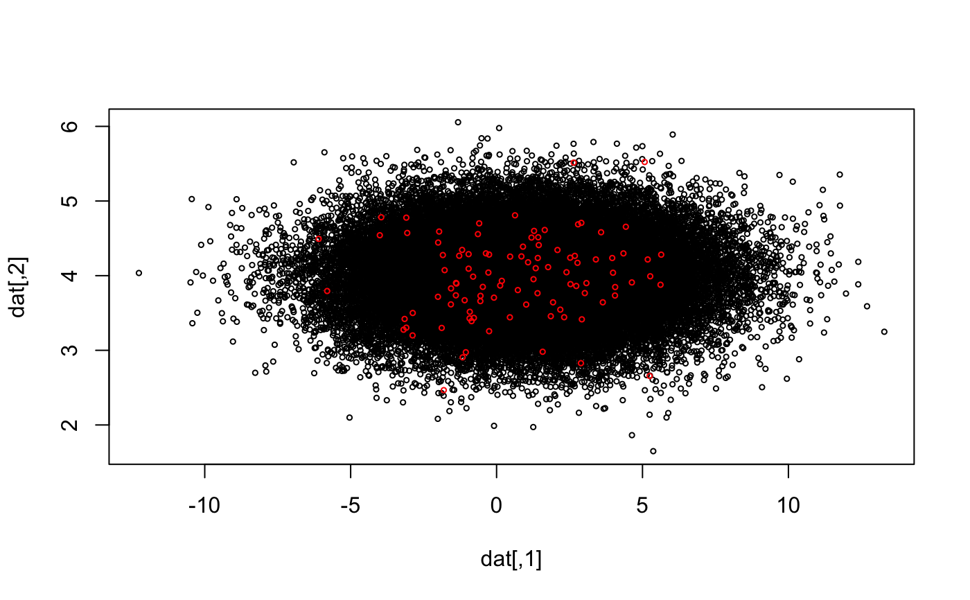
Examples

# simulate data and plot it
n = 5e4
dat = cbind(rnorm(n, mean = 1, sd = 3),
            rnorm(n, mean=4, sd = 0.5))
plot(dat, cex=0.5)
# fit Gaussian Copula
temp.cop = gcopFit(X = dat, fitXD = "kernel")
# simulate data from Copula model and add it to plot, should blend in
new.data = rgcop(100, temp.cop)
points(new.data, cex = 0.5, col="red")