Introduction to subdiff: Tools for the Analysis of Passive Particle-Tracking Data

Martin Lysy, Yun Ling

2024-09-06

Introduction

The subdiff package provides a number of utilities for analyzing subdiffusion in passive particle tracking data. Let \(\boldsymbol{X}(t) = \big(X_1(t), \ldots, X_{d}(t)\big)\) denote the \(d\)-dimensional position of a particle at time \(t\), where \(d\) is typically between 1 and 3. In an ideal experiment, it is typically assumed that \(\boldsymbol{X}(t)\) is a Continuous Stationary Increments (CSI) process, i.e., a stochastic process with mean zero and such that the distribution of \(\Delta\boldsymbol{X}(t) = \boldsymbol{X}(t+\Delta t) - \boldsymbol{X}(t)\) is independent of \(t\). Under these conditions, the covariance properties of \(\boldsymbol{X}(t)\) can often be deduced entirely from the particle’s mean square displacement (MSD), \[\begin{equation} \operatorname{MSD}_{\boldsymbol{X}}(t) = \sum_{i=1}^dE\big[\big(X_i(t)-X_i(0)\big)^2\big]. \tag{1} \end{equation}\] A widely observed phenomenon is that the MSD of microparticles diffusing in biological fluids has a power-law signature on a given timescale, \[\begin{equation} \operatorname{MSD}_{\boldsymbol{X}}(t) \sim 2dD \cdot t^\alpha, \qquad t \in (t_{\textrm{min}}, t_{\textrm{max}}). \tag{2} \end{equation}\] Whereas \(\alpha = 1\) corresponds to the MSD of ordinary diffusion observed in Brownian particles, the power law MSD (2) with \(\alpha \in (0,1)\) is referred to as subdiffusion.

The purpose of the subdiff library is to provide simple and computationally efficient tools for modeling and estimating subdiffusion. An overview of these tools is presented below.

Installation

To install the subdiff package:

1. Install the Rcpp package. To do this properly you will also need to install a C++ compiler. Instructions for this are available here.

   To test that this step is done correctly, quit + restart R, then run the following command:

   Rcpp::evalCpp("2 + 2")

   If the output is 4 then Rcpp is installed correctly.

2. Install the devtools package.

3. In an R session run the following commands:

   devtools::install_github("mlysy/subdiff",
                            force = TRUE, INSTALL_opts = "--install-tests")

4. Once the packages are installed, to test that everything works correctly, quit + restart R then run the command:

   testthat::test_package("subdiff", reporter = "progress")

   Occasionally due to random chance a few of the tests may fail. However, if everything works correctly then rerunning this a few times will eventually produce zero test failures.

Dataset

# load required packages
require(subdiff)
require(tidyr)
require(dplyr)
require(optimCheck)
require(ggplot2)
require(gridExtra)
## require(RColorBrewer)
## require(parallel)

Throughout, we’ll be using the hbe dataset included in the subdiff package, which consists of 76 2D trajectories of 1-micron tracer particles in 2.5 wt% mucus harvested from human bronchial epithelial (HBE) cell cultures, as detailed in Hill et al. (2014). Each trajectory contains 1102-1785 observations recorded at a frequency of 60Hz. The full dataset is displayed in Figure 1.

npaths <- length(unique(hbe$id)) # number of trajectories
n_rng <- range(tapply(hbe$id, hbe$id, length)) # range of trajectory lengths
dt <- 1/60 # interobservation time

# scatterplot of trajectories
hbe %>%
  ggplot(aes(x = x, y = y, group = id)) +
  geom_line(aes(color = id)) +
  xlab(expression("X Position ("*mu*m*")")) +
  ylab(expression("Y Position ("*mu*m*")")) +
  theme(legend.position = "none")
# histogram of trajectory lengths
hbe %>%
  group_by(id) %>%
  summarize(nobs = n(), .groups = "drop") %>%
  ggplot(aes(x = nobs)) +
  geom_histogram(bins = 30) +
  xlab("Number of Observations") +
  ylab("Counts")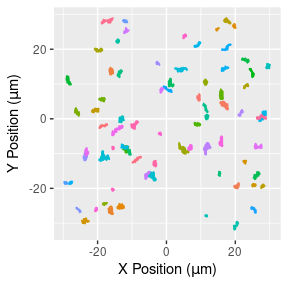

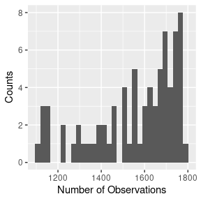
Figure 1: 2D particle trajectories (left) and number of observation in each (right).

Semiparametric Modeling

Let \(\boldsymbol{X}_n = \boldsymbol{X}(t_n)\) denote the position of a givne particle at time \(t_n = n \cdot \Delta t\), such that the data for the entire trajectory is given by \(\boldsymbol{X}= (\boldsymbol{X}_{0},\ldots,\boldsymbol{X}_{N})\). The semi-parametric subdiffusion estimator consists of two steps:

1. Calculate the empirical MSD for each trajectory, defined as

   \[\begin{equation} \widehat{\operatorname{MSD}}_{\boldsymbol{X}}(t_n) = \frac 1 {(N-n+1)} \sum_{h=0}^{N-n} \Vert \boldsymbol{X}_{h+n}-\boldsymbol{X}_{h}\Vert^2. \tag{3} \end{equation}\]

2. Estimate \((\alpha,D)\) by regressing \(y_n = \log \widehat{\operatorname{MSD}}_{\boldsymbol{X}}(t_n)\) onto \(x_n = \log t_n\), such that

   \[ \hat \alpha = \frac{\sum_{n=0}^N(y_n - \bar y)(x_n - \bar x)}{\sum_{n=0}^N(x_n - \bar x)^2}, \qquad \hat D = \frac 1 {2d} \exp(\bar y - \hat \alpha \bar x), \]

   where \(\bar x\) and \(\bar y\) are the samples means of \(x_n\) and \(y_n\).

Since particle trajectories are often contaminated with low-frequency drift, the empirical MSD is often calculated on the drift-subtracted observations,

\[ \tilde{\boldsymbol{X}}_n = \boldsymbol{X}_n - \hat{\boldsymbol{\mu}} \cdot t_n, \]

where \(\hat{\boldsymbol{\mu}} = (\hat \mu_1, \ldots, \hat \mu_{d})\) is the vector of slope terms of the linear regression of \(\boldsymbol{X}\) onto \(\boldsymbol{t} = (t_{0},\ldots,t_{N})\). Morever, the empirical MSD is known to be biased at large lag times, such that only about 30-50% of the shortest lagtimes are usually kept for estimating \((\alpha,D)\).

Figure 2 displays the empirical MSD of the first 500 lags for each trajectory and the corresponding estimates of \((\alpha,D)\).

# calculate empirical MSDs
ids <- unique(hbe$id)
nlag <- 500 # number of lags
dt <- 1/60 # interobservation time
tseq <- 1:nlag*dt # time sequence
msd_hat <- lapply(ids, function(id) {
  Xt <- hbe %>%
    filter(id == !!id) %>%
    select(x, y)
  tibble(id = id, t = tseq, msd = msd_fit(Xt = Xt, nlag = nlag))
}) %>% bind_rows()

# calculate mean MSD and its standard error
msd_stats <- msd_hat %>%
  group_by(t) %>%
  summarize(est = mean(msd),
            se = sd(msd) / sqrt(n()),
            .groups = "drop")

# plot msd's with mean +/- 1.96 se
ggplot(data = msd_stats) +
  # individual msd's
  geom_line(data = msd_hat,
            mapping = aes(x = t, y = msd, group = factor(id),
                          color = "msd")) +
  # +/- 1.96*se confidence band
  geom_ribbon(mapping = aes(x = t,
                            ymin = est-1.96*se, ymax = est+1.96*se,
                            color = "se", fill = "se", alpha = "se")) +
  # mean line
  geom_line(aes(x = t, y = est, color = "est")) +
  # set colors manually
  scale_color_manual(values = c(msd = "lightblue", est = "black", se = NA)) +
  scale_fill_manual(values = c(msd = NA, est = NA, se = "red")) +
  scale_alpha_manual(values = c(msd = NA, est = NA, se = .5)) +
  # axes names and log-scale
  scale_x_continuous(name = expression("Time (s)"), trans = "log10") +
  scale_y_continuous(name = expression("MSD ("*mu*m^2*")"), trans = "log10") +
  # remove legend
  theme(legend.position = "none")

# estimate & plot subdiffusion parameters
aD_hat <- lapply(ids, function(id) {
  Xt <- hbe %>%
    filter(id == !!id) %>%
    select(x, y)
  ls_fit(Xt, dt = dt, lags = 1:nlag, vcov = FALSE)
}) %>% bind_rows() 

aD_hat %>%  
  ggplot(aes(x = exp(logD), y = alpha)) +
  geom_point() + 
  xlab(expression("D")) +
  ylab(expression(alpha)) +
  scale_x_log10()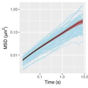

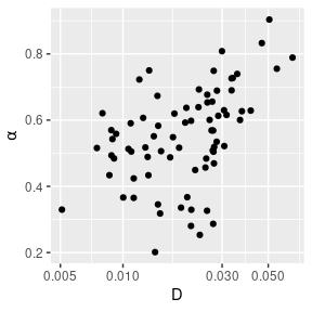
Figure 2: Empirical MSDs for the 76 trajectories (left) and corresponding estimates of \((\alpha,D)\) (right).

Parametric Modeling with Fractional Brownian Motion

In addition to the semiparameteric “least-squares” (LS) estimator presented above, subdiff offers a range of fully-parametric subdiffusion modeling options. To illustrate, let’s start with a basic model in which the particle trajectory \(\boldsymbol{X}(t)\) is given by \[\begin{equation} \boldsymbol{X}(t) = \boldsymbol{\mu}\cdot t + \boldsymbol{\Sigma}^{1/2} \boldsymbol{B}^{(\alpha)}(t), \tag{4} \end{equation}\] where:

• \(\boldsymbol{\mu}= (\mu_1, \ldots, \mu_{d})\) is the linear drift velocity per coordinate.

• \(\boldsymbol{\Sigma}\) is a \(d\times d\) symmetric positive-definite scaling matrix.

• \(\boldsymbol{B}^{(\alpha)}(t) = \big(B_1^{(\alpha)}(t), \ldots, B_{d}^{(\alpha)}(t)\big)\) are independent and identically distributed (iid) copies of a fractional Brownian motion (fBM) process \(B^{(\alpha)}(t)\). That is, fBM is the only Gaussian CSI process with MSD

  \[ \operatorname{MSD}_{B^{(\alpha)}}(t) = t^\alpha. \]

An attractive feature of model (4) is that the MSD of the drift-subtracted particle trajectory \(\tilde{\boldsymbol{X}}(t) = \boldsymbol{X}(t) - t \boldsymbol{\mu}= \boldsymbol{\Sigma}^{1/2} \boldsymbol{B}^{(\alpha)}(t)\) is simply given by \[ \operatorname{MSD}_{\tilde{\boldsymbol{X}}} = \operatorname{trace}(\boldsymbol{\Sigma}) \cdot t^{\alpha}, \] such that \(D = \operatorname{trace}(\boldsymbol{\Sigma})/(2d)\). The MLE \((\hat \alpha, \log \hat D)\) for \((\alpha, \log D)\) and the corresponding variance estimator \(\hat V = \widehat{\operatorname{var}}(\hat \alpha, \log \hat D)\) for each trajectory can be computed with subdiff::fbm_fit():

# extract a single trajectory
Xt <- hbe %>%
  filter(id == 1) %>%
  select(x, y) %>%
  as.matrix()

# fit fbm to data
fbm_est <- fbm_fit(Xt = Xt, dt = dt, drift = "linear")
fbm_est
#> $coef
#>      alpha       logD 
#>  0.7432851 -3.4418462 
#> 
#> $vcov
#>              alpha        logD
#> alpha 0.0005982074 0.002275383
#> logD  0.0022753833 0.009387893

But what about estimates of the full set of parameters, \(\boldsymbol{\theta}= (\alpha, \boldsymbol{\mu}, \boldsymbol{\Sigma})\)? We’ll return to this point below.

Parametric Modeling in the Presense of Noise

Figure 3 displays MSD estimates for the trajectory Xt above, using the (drift-subtracted) empirical estimator (3) and that of the fitted fBM model.

tmax <- 10 # seconds
Nmax <- floor(tmax/dt)

tibble(t = 1:Nmax * dt,
       Empirical = msd_fit(Xt, nlag = Nmax),
       fBM = 4 * exp(fbm_est$coef["logD"]) * (1:Nmax * dt)^fbm_est$coef["alpha"]) %>%
  pivot_longer(cols = Empirical:fBM, names_to = "MSD Type", values_to = "msd") %>%
  ggplot(aes(x = t, y = msd, group = `MSD Type`)) +
  geom_line(aes(col = `MSD Type`)) +
  scale_x_continuous(name = expression("Time (s)"), trans = "log10") +
  scale_y_continuous(name = expression("MSD ("*mu*m^2*")"), trans = "log10")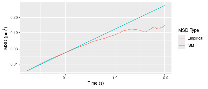  

Figure 3: Empirical and fBM-fitted MSDs.

Figure 3 shows that the empirical MSD has an inflection point around 0.05 seconds, which we also see in the average MSD (over all 76 trajectories) in Figure 2. This is not a feature of the underlying particle motion, but rather of various sources of experimental noise due to e.g.: mechanical vibrations of the instrumental setup; particle displacement while the camera shutter is open; noisy estimation of true position from the pixelated microscopy image; and error-prone tracking of particle positions when they are out of the camera focal plane.

The subdiff package currently provides two parametric models to account for the high-frequency “localization errors” described above. The first relies on a physical characterization of the localization errors given in the seminal paper of Savin and Doyle (2005). For a one dimensional particle trajectory \(X(t)\), let \(Y_n\) denote the measured position at time \(t_n = n \cdot \Delta t\). The Savin-Doyle model for \(Y_n\) is

\[\begin{equation} Y_n = \frac 1 \tau \int_0^{\tau} X(t_n - s) \mathop{}\!\mathrm{d}s + \varepsilon_n, \tag{5} \end{equation}\]

where \(\varepsilon_n \stackrel{\mathrm{iid}}{\sim}\mathcal{N}(0, \sigma^2)\) represents the “static” noise due to measurement error in recording the position of the particle at a given time, and the integral term represents the “dynamic” noise due to movement of the particle during the camera exposure time \(0 < \tau < \Delta t\).

The second parametric noise model provided by subdiff is that of Ling et al. (2022). Rather than attempting to characterize the complex physics of the localization errors, the strategy here is to provide sufficient modeling flexibility to capture any high-frequency errors exhibited by the experimental data. This is achieved via the general family of \(\operatorname{ARMA}(p, q)\) models, such that the measurements \(Y_n\) related to the true positions \(X_n = X(t_n)\) via

\[\begin{equation} Y_n = \sum_{i=1}^p \theta_i Y_{n-i} + \sum_{j=0}^q \rho_j X_{n-j}, \end{equation}\]

where we have the parameter restriction \(\rho_0 = 1 - \sum_{i=1}^p \theta_i - \sum_{j=1}^q \rho_j\). To illustrate the difference between the two noise models, suppose that \(X(t) = D \cdot B^{(\alpha)}(t)\) is an fBM process with \(\alpha = 0.8\) and \(D = 1\). The MSD of the corresponding fBM-driven Savin-Doyle model (5), which we call fSD, is plotted in Figure 4(a), with different values of the noise parameters. Here, we parametrize the static error by the signal-to-noise ratio, \(\mathrm{SNR}= \operatorname{var}(X(\Delta t))/\sigma^2 = D \Delta t^\alpha / \sigma^2\). Figure 4(b) displays the MSD of the simplest fBM-driven \(\operatorname{ARMA}(p,q)\) model, a purely moving-average model with \(p = 0\) and \(q = 1\):

\[ Y_n = (1-\rho) X_n + \rho X_{n-1}. \]

We call this model fMA. Figure 4(b) plots its MSD over the valid parameter range \(-1 \le \rho \le 0.5\) (see Appendix for code).

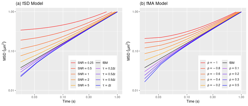
Figure 4: MSDs of the fSD and fMA models with different noise parameter values.

As we can see, the fSD model is more expressive for localization errors which inflate the MSD at shorter timescales, while fMA is more expressive errors which suppress it. The following code fits the fSD and fMA models, and compare their estimates to fBM without error correction.

# fit fsd to data
fsd_est <- fsd_fit(Xt = Xt, dt = dt, drift = "linear")
# fit fma to data
fma_est <- farma_fit(Xt = Xt, dt = dt, order = c(0, 1), drift = "linear")

# display nicely

# display estimates and standard errors for (alpha, logD) 
to_summary <- function(est) {
  coef <- est$coef
  se <- setNames(sqrt(diag(est$vcov)), nm = paste0(names(coef), "_se"))
  c(coef[1], se[1], coef[2], se[2])
}
disp <- rbind(fbm = to_summary(fbm_est),
              fsd = to_summary(fsd_est),
              fma = to_summary(fma_est))
signif(disp, 2)
#>     alpha alpha_se logD logD_se
#> fbm  0.74    0.024 -3.4   0.097
#> fsd  0.55    0.048 -3.8   0.096
#> fma  0.59    0.037 -3.7   0.099

These numbers indicate that the \((\alpha,D)\) estimates with noise correction are more than two standard errors away from those of pure fBM.

User-Defined Models

The subdiff tools can be applied to a large family of user-defined models. These are based on the location-scale modeling framework of Lysy et al. (2016), whereby the particle trajectory \(\boldsymbol{X}(t)\) is given by \[\begin{equation} \boldsymbol{X}(t) = \boldsymbol{R}(t \mid \boldsymbol{\phi})' \boldsymbol{\mu}+ \boldsymbol{\Sigma}^{1/2} \boldsymbol{Z}(t), \tag{6} \end{equation}\] where:

• \(\boldsymbol{Z}(t) = \big(Z_1(t), \ldots, Z_{d}(t)\big)\) are independent and identically distributed (iid) copies of a CSI process \(Z(t)\) having MSD

  \[ \operatorname{MSD}_Z(t) = \eta(t \mid \boldsymbol{\phi}). \]

• \(\boldsymbol{\Sigma}\) is a \(d\times d\) symmetric positive-definite scaling matrix.

• \(\boldsymbol{R}(t \mid \boldsymbol{\phi}) = \big( R_1(t \mid \boldsymbol{\phi}), \ldots, R_{k}(t \mid \boldsymbol{\phi}) \big)\) is a set of \(k\) drift basis functions. Typically it will be linear or quadratic, corresponding to \(\boldsymbol{R}(t) = t\) and \(\boldsymbol{R}(t) = (t, t^2)\) with \(k= 1\) and \(k= 2\), respectively. However, subdiff allows for an arbitrary number of basis functions possibly dependent on the “kernel” parameters \(\boldsymbol{\phi}\).

• \(\boldsymbol{\mu}\) is \(k\times d\) matrix of drift coefficients. For linear drift, \(\boldsymbol{\mu}= (\mu _{1},\ldots,\mu _{d})\) correspond to per-coordinate drift velocities.

An attractive feature of model (6) is that the MSD of the drift-subtracted particle trajectory \(\tilde{\boldsymbol{X}}(t) = \boldsymbol{X}(t) - \boldsymbol{R}(t)' \boldsymbol{\mu}\) has the simple formula

\[ \operatorname{MSD}_{\tilde{\boldsymbol{X}}} = \operatorname{trace}(\boldsymbol{\Sigma}) \cdot \eta(t \mid \boldsymbol{\phi}). \]

Another appealing property of this model is that its parameters \(\boldsymbol{\theta}= (\boldsymbol{\phi}, \boldsymbol{\mu}, \boldsymbol{\Sigma})\) can be estimated from discrete observations \(\boldsymbol{X}= (\boldsymbol{X}_{0},\ldots,\boldsymbol{X}_{N})\) in a computationally efficient manner (Ling and Lysy 2020).

Example: Brownian Motion in a Jeffreys Fluid

Consider a particle of radius \(r\) in a Jeffreys fluid described by viscosity parameters \(\eta_1\) and \(\eta_2\) and elastic modulus \(\Gamma\). The MSD of the drift-subtracted particle trajectory \(\tilde{\boldsymbol{X}}(t)\) is given by (Raikher and Rusakov 2010)

\[\begin{equation} \operatorname{MSD}_{\tilde{\boldsymbol{X}}}(t) = \frac{2dk_{\mathrm{B}}T}{\xi_V(1+q)} \times \left\{t + \frac{q}{1+q} \tau_M \left[1 - \exp\left(-\frac{(1+q)t}{\tau_M}\right)\right]\right\}, \tag{7} \end{equation}\]

where \(q = \eta_1/\eta_2\), \(\tau_M = (\eta_1 + \eta_2)/\Gamma\), \(\xi_V = 6\pi r \cdot \eta_1\eta_2/(\eta_1 + \eta_2)\), and \(T\) and \(r\) are the temperature of the system and radius of the particle, respectively. A more natural parametrization is

\[ \operatorname{MSD}_{\tilde{\boldsymbol{X}}}(t) = 2d\sigma^2 \left\{t + \alpha \left[1 - e^{-t/\tau}\right]\right\}, \]

where \(\tau = \tau_M/(1+q) = \eta_2/\Gamma\), \(\alpha = \tau q = \eta_1/\Gamma\), and \(\sigma^2 = k_{\mathrm{B}}T/ (\xi_V(1+q)) = k_{\mathrm{B}}T/ (6\pi r \eta_1)\). In the formulation of the location-scale model (6), the CSI process \(Z(t)\) underlying the particle trajectory \(\boldsymbol{X}(t)\) has MSD

\[ \eta(t \mid \boldsymbol{\phi}) = \operatorname{MSD}_Z(t) = \left\{t + \alpha \left[1 - e^{-t/\tau}\right]\right\} \]

with \(\boldsymbol{\phi}= (\alpha, \tau)\), and the MSD scale factor is \(\sigma^2 = \operatorname{trace}(\boldsymbol{\Sigma})/(2d)\).

Creating the Jeffreys Model Class

In order to fit the Jeffreys model (7) to trajectory data, we will create a class jfs_model which will derive from the base class csi_model used to represent the general location-scale model (6). In order to do this, we will need the following ingredients:

• The increment autocorrelation function

  \[ \operatorname{ACF}_{\Delta Z}(h) = \operatorname{cov}(\Delta Z_n, \Delta Z_{n+h}). \]

  This must be supplied as a function with arguments \((\boldsymbol{\phi}, \Delta t, N)\) and return the vector \(\big(\operatorname{ACF}_{\Delta Z}(0), \ldots, \operatorname{ACF}_{\Delta Z}(N-1)\big)\). Note that \(\operatorname{MSD}_{Z}(t)\) can be converted to \(\operatorname{ACF}_{\Delta Z}(h)\) via the function SuperGauss::msd2acf(), as we do in the function jfs_acf() below.

• Functions to convert back and forth between the kernel parameters in the “inferential” basis, \(\boldsymbol{\phi}\), and these parameters in a “computational basis”, \(\boldsymbol{\psi}\). That is, \(\boldsymbol{\psi}\) should have the same dimension as \(\boldsymbol{\phi}\) but have no constraints. For the Jeffreys model, since \(\alpha, \tau > 0\), a natural choice of computational basis is \(\boldsymbol{\psi}= (\log \alpha, \log \tau)\).

• Specification of the drift basis functions \(\boldsymbol{R}(t \mid \boldsymbol{\phi})\). This is done automatically in the case of linear, quadratic, or no drift, so we’ll skip this here.

• A character vector of the names of the elements of \(\boldsymbol{\phi}\) for display purposes.

The following code block defines the jfs_model class. This is done with the R6 class mechanism, of which a basic understanding is assumed. More information about the base class for location-scale models can be obtained from the package documentation: ?csi_model.

#' Calculate the ACF of the Jeffreys model.
#'
#' @param alpha Scale parameter.
#' @param tau Decorrelation time.
#' @param dt Interobservation time.
#' @param N Number of ACF lags to return.
#'
#' @return An ACF vector of length `N`.
jfs_acf <- function(alpha, tau, dt, N) {
  t <- (1:N)*dt # time vector
  msd <- (t + alpha * (1 - exp(-t/tau)))
  SuperGauss::msd2acf(msd) # convert msd to acf
}

jfs_model <- R6::R6Class(
  classname = "jfs_model",
  inherit = subdiff::csi_model,

  public = list(
    # Kernel parameter names in the inferential basis.
    phi_names = c("alpha", "tau"),

    # Autocorrelation function.
    acf = function(phi, dt, N) {
      jfs_acf(alpha = phi[1], tau = phi[2], dt = dt, N = N)
    },

    # Transform kernel parameters from inferential to computational basis.
    trans = function(phi) {
      psi <- log(phi)
      names(psi) <- private$psi_names # these are determined automatically.
      psi
    },

    # Transform kernel parameters from computational to inferential basis.
    itrans = function(psi) {
      phi <- exp(psi)
      names(phi) <- self$phi_names
      phi
    }
  )
)

Simulation

The following code shows how to simulate the trajectory of a particle from the Jeffreys model with parameters \(\tau_M = 2.1\, \mathrm{s}\), \(q = 46\), and \(\xi_V = 1.4\times 10^{-7}\, \mathrm{kg/s}\) and temperature \(T = 298\, \mathrm{K}\). The 2D trajectory is generated with zero drift \(\boldsymbol{R}(t \mid \boldsymbol{\phi}) = 0\), and scale factor \(\boldsymbol{\Sigma}= \left[\begin{smallmatrix} \sigma^2 & 0 \\ 0 & \sigma^2 \end{smallmatrix} \right]\). Figure 5 compares the empirical MSD for the simulated trajectory to the theoretical MSD.

kB <- 1.38064852e-23 # Boltzmann constant

# simulation parameters
tau_M <- 2.1 # seconds
q <- 4.6e1 # unitless
xi_V <- 1.4e-07 # kg/s
Temp <- 298 # temperature of the system (Kelvin)

dt <- 1/60 # interobservation time
N <- 1800 # number of observations
ndim <- 2 # number of dimensions

# increment autocorrelation
tau <- tau_M/(1+q)
alpha <- tau * q
acf <- jfs_acf(alpha = alpha, tau = tau, dt = dt, N = N)
# increment drift matrix: in this case zero drift
drift <- matrix(0, N, ndim)
# scale matrix (micron^2)
sigma2 <- 1e12 * kB*Temp / (xi_V * (1+q))
Sigma <- sigma2 * diag(ndim)
# position at time t = 0
X0 <- rep(0, ndim)

# generate data
Xt <- csi_sim(drift = drift, acf = acf,
              Sigma = Sigma, X0 = X0)

# plot empirical and theoretical MSD
tmax <- 10 # maximum time to plot
nmax <- floor(tmax/dt) # corresponding MSD lag number
tibble(
  Time = 1:nmax * dt, # time sequence
  Theoretical = ndim*sigma2 * SuperGauss::acf2msd(acf[1:nmax]), # theoretical msd
  Empirical = msd_fit(Xt, nlag = nmax) # empirical msd
) %>%
  pivot_longer(cols = Theoretical:Empirical, names_to = "MSD Type",
               values_to = "MSD") %>%
  mutate(`MSD Type` = factor(`MSD Type`)) %>%
  ggplot(aes(x = Time, y = MSD, group = `MSD Type`)) +
  geom_line(aes(color = `MSD Type`)) +
  scale_x_log10() + scale_y_log10() +
  xlab(expression("Time "*(s))) + ylab(expression("MSD "*(mu*m^2)))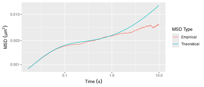

Figure 5: Empirical and theoretical MSD for the Jeffreys model with parameters \(\tau_M = 2.1\, \mathrm{s}\), \(q = 46\), and \(\xi_V = 1.4\times 10^{-7}\, \mathrm{kg/s}\) and temperature \(T = 298\, \mathrm{K}\).

Parameter Estimation

The jfs_model class inherits from the base class csi_model, which contains a number of methods to assist with parameter estimation. In the following example, we’ll use these to calculate the MLE of the Jeffreys fluid parameters \(\boldsymbol{\zeta}= (\eta_1, \eta_2, \Gamma)\) along with their standard errors. This proceeds in several steps:

Step 1: Profile Likelihood

The first step is to calculate the MLE of the kernel parameters \(\boldsymbol{\phi}= (\alpha, \tau)\). Let \(\ell(\boldsymbol{\theta}\mid \boldsymbol{X}) = \ell(\boldsymbol{\phi}, \boldsymbol{\mu}, \boldsymbol{\Sigma}\mid \boldsymbol{X})\) denote the loglikelihood function for the complete set of parameters. As noted in Ling et al. (2022),

\[ (\hat{\boldsymbol{\mu}}_{\boldsymbol{\phi}}, \hat{\boldsymbol{\Sigma}}_{\boldsymbol{\phi}}) = \operatorname{arg\,max}_{(\boldsymbol{\mu}, \boldsymbol{\Sigma})} \ell(\boldsymbol{\phi}, \boldsymbol{\mu}, \boldsymbol{\Sigma}\mid \boldsymbol{X}) \]

is available in closed-form, from which we may calculate the so-called profile likelihood function

\[\begin{equation} \begin{aligned} \ell_{\textrm{prof}}(\boldsymbol{\phi}\mid \boldsymbol{X}) &= \max_{\boldsymbol{\mu}, \boldsymbol{\Sigma}} \ell(\boldsymbol{\phi}, \boldsymbol{\mu}, \boldsymbol{\Sigma}\mid \boldsymbol{X}) \\ & = \ell(\boldsymbol{\phi}, \hat{\boldsymbol{\mu}}_{\boldsymbol{\phi}}, \hat{\boldsymbol{\Sigma}}_{\boldsymbol{\phi}} \mid \boldsymbol{X}). \end{aligned} \tag{8} \end{equation}\]

It follows that if \(\hat{\boldsymbol{\phi}} = \operatorname{arg\,max}_{\boldsymbol{\phi}} \ell_{\textrm{prof}}(\boldsymbol{\phi}\mid \boldsymbol{X})\), then the MLE of \(\boldsymbol{\theta}= (\boldsymbol{\phi}, \boldsymbol{\mu}, \boldsymbol{\Sigma})\) is given by

\[ \hat{\boldsymbol{\theta}} = (\hat{\boldsymbol{\phi}}, \hat{\boldsymbol{\mu}}_{\hat{\boldsymbol{\phi}}}, \hat{\boldsymbol{\Sigma}}_{\hat{\boldsymbol{\phi}}}). \]

The upshot of this technique is that \(\hat{\boldsymbol{\theta}}\) can be obtained by maximizing \(\ell_{\textrm{prof}}(\boldsymbol{\phi}\mid \boldsymbol{X})\) rather than \(\ell(\boldsymbol{\theta}\mid \boldsymbol{X})\). The former is a lower-dimensional optimization problem, and thus more computationally efficient.

The following code shows how to calculate \(\hat{\boldsymbol{\theta}}\). Note that the optimization of the profile likelihood (8) is done with respect to \(\boldsymbol{\psi}\), the kernel parameters in the computational basis. We’ll use the function stats::optim() for this.

# construct the model object
mod <- jfs_model$new(Xt = Xt, dt = dt)

# minimize the negative profile likelihood.
opt <- optim(fn = mod$nlp, # negative profile likelihood
             par = c(0, 0)) # initial value of psi

# mle of psi
psi_hat <- opt$par
psi_hat
#> [1]  0.4958942 -3.2063559

Before going further, it is sometimes useful to check whether stats::optim() has indeed converged. One way to do this is by examining the convergence flag:

opt$convergence
#> [1] 0

A value of zero means stats::optim() thinks it has converged. Any other value means it hasn’t converged (details in the function documentation). However, the convergence metric used by stats::optim() is sometimes unreliable. A more reliable but slower convergence diagnostic is to look at projection plots. The process is facilitated with the use of the R package optimCheck.

optimCheck::optim_proj(fun = mod$nlp, # function to minimize
                       xsol = psi_hat, # candidate for local minimum
                       xnames = expression(log(alpha), log(tau)), # parameter names
                       maximum = FALSE) # check minimum not maximum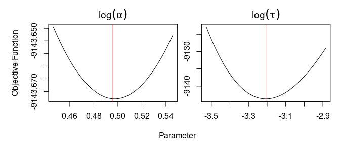

Figure 6: Projection plots for profile likelihood maximization. Red lines correspond to values of the candidate solution.

The red lines in Figure 6 correspond to the values of the candidate solution \(\boldsymbol{\psi}\). The fact that each of these values is at the minimum of the projection plot of the corresponding negative profile loglikelihood function indicates that stats::optim() has found a local optimum. We can now convert \(\hat{\boldsymbol{\psi}}\) into the MLE of \(\boldsymbol{\theta}\):

phi_hat <- mod$itrans(psi = psi_hat) # convert psi to inferential basis (phi)
nu_hat <- mod$nu_hat(phi = phi_hat) # calculate nu_hat = (mu_hat, Sigma_hat)
theta_hat <- list(phi = phi_hat, mu = nu_hat$mu, Sigma = nu_hat$Sigma)
theta_hat
#> $phi
#>      alpha        tau 
#> 1.64196583 0.04050394 
#> 
#> $mu
#>             [,1]         [,2]
#> [1,] 0.004414467 0.0006510514
#> 
#> $Sigma
#>              [,1]         [,2]
#> [1,] 6.951635e-04 6.862189e-06
#> [2,] 6.862189e-06 7.556147e-04

Step 2: Variance Estimation

The variance of the MLE, \(\operatorname{var}(\hat{\boldsymbol{\theta}})\), is estimated by \(\boldsymbol{V}(\hat{\boldsymbol{\theta}})\), the inverse of the observed Fisher information matrix,

\[ \boldsymbol{V}(\hat{\boldsymbol{\theta}}) = \left[- \frac{\partial^2}{\partial \boldsymbol{\theta}\partial \boldsymbol{\theta}'} \ell(\hat{\boldsymbol{\theta}} \mid \boldsymbol{X})\right]^{-1}. \]

The confidence interval for a given parameter \(\theta_j\) is then given by \(\hat \theta_j \pm 2 \operatorname{se}(\hat \theta_j)\), where the standard error is \(\operatorname{se}(\hat \theta_j) = \sqrt{[\boldsymbol{V}(\hat{\boldsymbol{\theta}})]_{jj}}\).

The subdiff package calculates the variance estimate using numerical differentiation via the R package numDeriv. However, rather than calculating the Hessian of the loglikelihood with respect to the inferential basis \(\boldsymbol{\theta}\), subdiff instead does this with respect to a computational basis \(\boldsymbol{\omega}= (\boldsymbol{\psi}, \boldsymbol{\mu}, \boldsymbol{\lambda})\), where \(\boldsymbol{\lambda}\) is the log-Cholesky decomposition of \(\boldsymbol{\Sigma}\). That is, for \(\boldsymbol{\Sigma}_{d\times d}\), \(\boldsymbol{\lambda}\) is a vector of size \(d(d+1)/2\) corresponding to the upper Cholesky factor of \(\boldsymbol{\Sigma}\) in column-major order, but with the log of its diagonal elements. In other words, if \[ \boldsymbol{U}_{d\times d} = \begin{bmatrix} \exp(\lambda_1) & \lambda_2 & \cdots & \lambda_{d(d-1)/2 + 1} \\ 0 & \exp(\lambda_3) & \cdots & \lambda_{d(d-1)/2 + 2} \\ \vdots & & \ddots & \vdots \\ 0 & 0 & \cdots & \exp(\lambda_{d(d-1)/2+d}) \end{bmatrix}, \] then \(\boldsymbol{U}\) is the unique upper-triangular matrix with positive diagonal elements such that \(\boldsymbol{\Sigma}= \boldsymbol{U}'\boldsymbol{U}\). The vector \(\boldsymbol{\lambda}\) is unconstrained in \(\mathbb{R}^{d(d-1)/2+d}\), and consequently \(\boldsymbol{\omega}\) is unconstrained in \(\mathbb{R}^{\operatorname{dim}(\boldsymbol{\omega})}\) as well, which make the numerical Hessian calculation more stable and more accurate. Moreover, the estimators \(\hat{\boldsymbol{\omega}}\) and \(\boldsymbol{V}(\hat{\boldsymbol{\omega}})\) can be easily used to calculate standard errors and confidence intervals for any parameter of interest as we shall see below.

The following R code shows how to calculate \(\hat{\boldsymbol{\omega}}\) and \(\boldsymbol{V}(\hat{\boldsymbol{\omega}})\).

# convert theta to computational basis (omega)
omega_hat <- mod$trans_full(phi = theta_hat$phi,
                            mu = theta_hat$mu,
                            Sigma = theta_hat$Sigma)
# calculate fisher information matrix
fi_obs <- mod$fisher(omega_hat)
# stable inversion of fisher information
omega_var <- mod$get_vcov(fi_obs)
list(coef = signif(omega_hat, 2),
     vcov = signif(omega_var, 2))
#> $coef
#>     psi1     psi2     mu11     mu12 lambda11 lambda12 lambda22 
#>  0.50000 -3.20000  0.00440  0.00065 -3.60000  0.00026 -3.60000 
#> 
#> $vcov
#>              psi1     psi2     mu11     mu12 lambda11 lambda12 lambda22
#> psi1      7.3e-02  1.1e-02 -2.7e-05 -4.9e-05 -3.1e-02 -2.0e-06 -3.1e-02
#> psi2      1.1e-02  4.6e-03 -4.0e-06 -8.3e-06 -3.7e-03  2.4e-07 -3.7e-03
#> mu11     -2.7e-05 -4.0e-06  2.4e-05  2.5e-07  1.2e-05  7.6e-10  1.2e-05
#> mu12     -4.9e-05 -8.3e-06  2.5e-07  2.6e-05  2.1e-05  1.2e-09  2.0e-05
#> lambda11 -3.1e-02 -3.7e-03  1.2e-05  2.1e-05  1.4e-02  1.1e-06  1.3e-02
#> lambda12 -2.0e-06  2.4e-07  7.6e-10  1.2e-09  1.1e-06  4.2e-07  1.0e-06
#> lambda22 -3.1e-02 -3.7e-03  1.2e-05  2.0e-05  1.3e-02  1.0e-06  1.4e-02

Step 3: Estimating Arbitrary Quantities of Interest

Let \(\boldsymbol{\psi}= (\psi_1, \ldots, \psi_P) \in \mathbb R^{P}\), for which we have the MLE \(\hat{\boldsymbol{\psi}}\) and its variance estimate \(\boldsymbol{V}(\hat{\boldsymbol{\psi}})\). Now suppose we wish to estimate the quantity of interest \(\boldsymbol{\zeta}= \boldsymbol{G}(\boldsymbol{\psi}) = \big(G_1(\boldsymbol{\psi}), \ldots, G_Q(\boldsymbol{\psi})\big) \in \mathbb R^{Q}\). Then the point estimate is \(\hat{\boldsymbol{\zeta}} = \boldsymbol{G}(\hat{\boldsymbol{\psi}})\), and the corresponding variance estimate is

\[ \boldsymbol{V}(\hat{\boldsymbol{\zeta}}) = \boldsymbol{J}(\hat{\boldsymbol{\psi}})' \boldsymbol{V}(\hat{\boldsymbol{\psi}}) \boldsymbol{J}(\hat{\boldsymbol{\psi}}), \]

where \(\boldsymbol{J}(\boldsymbol{\psi})\) is the \(P \times Q\) Jacobian matrix with elements \([\boldsymbol{J}(\boldsymbol{\psi})]_{ij} = \frac{\partial}{\partial \psi_i} G_j(\boldsymbol{\psi})\). The code below shows how to do this for the Jeffreys model parameters \(\boldsymbol{\zeta}= (\eta_1, \eta_2, \Gamma)\) for a particle of radius \(r = 0.48 \, \mu\mathrm{m}\) at temperature \(T = 298\, \mathrm{K}\). The Jacobian matrix \(\boldsymbol{J}(\hat{\boldsymbol{\psi}})\) is calculated numerically using numDeriv::jacobian().

#' Calculate the Jeffreys model parameters from the parameters of the computational basis.
#'
#' @param omega Vector of computational basis parameters.
#' @param model Jeffreys model object of class `jfs_model`.  This is used to convert `omega` to the inferential basis `theta = (phi, mu, Sigma)`.
#' @param rad Radius of the particle (m).
#' @param Temp Temperature of the system (Kelvin).
#' 
#' @return A vector with named elements `eta1` (N s / m^2), `eta2` (N s / m^2), and `Gamma` (kg / (m s^2)).
jfs_zeta <- function(omega, model, rad, Temp) {
  kB <- 1.38064852e-23 # Boltzmann constant: m^2 kg /(s^2 K)
  # convert omega to theta
  theta <- model$itrans_full(omega)
  # parameters in simplified basis
  alpha <- theta$phi["alpha"]
  tau <- theta$phi["tau"]
  sigma2 <- mean(diag(theta$Sigma)) * 1e-12 # convert from micron^2 to m^2
  # parameters in original basis
  eta1 <- 2*kB*Temp / (6*pi*rad * sigma2)
  Gamma <- eta1/alpha
  eta2 <- tau*Gamma
  setNames(c(eta1, eta2, Gamma), c("eta1", "eta2", "Gamma"))
}

# estimate of zeta

rad <- 0.48 # particle radius (micron)
Temp <- 298 # temperature of the system (Kelvin)

# point estimate
zeta_hat <- jfs_zeta(omega = omega_hat,
                     model = mod,
                     rad = rad * 1e-6, # micron -> m
                     Temp = Temp)

# variance estimate
# jacobian is returned as a matrix of size `length(zeta) x length(omega)`
jac <- numDeriv::jacobian(
                   func = function(omega) {
                     jfs_zeta(omega,
                              model = mod, rad = rad*1e-6, Temp = Temp)
                   },
                   x = omega_hat
                 )
zeta_var <- jac %*% omega_var %*% t(jac)
colnames(zeta_var) <- rownames(zeta_var) <- names(zeta_hat)

list(coef = signif(zeta_hat, 2),
     vcov = signif(zeta_var, 2))
#> $coef
#>  eta1  eta2 Gamma 
#> 1.300 0.031 0.760 
#> 
#> $vcov
#>           eta1     eta2    Gamma
#> eta1   8.5e-02 -7.7e-06 -7.3e-03
#> eta2  -7.7e-06  8.7e-07 -2.0e-06
#> Gamma -7.3e-03 -2.0e-06  2.0e-03

Finally we can convert the variance matrix estimate to standard errors and 95% confidence intervals for each element of \(\boldsymbol{\zeta}\).

# standard errors
zeta_se <- sqrt(diag(zeta_var))

# display point estimate, standard error, and confidence interval
disp <- cbind(est = zeta_hat,
              se = zeta_se,
              `2.5%` = zeta_hat - 2*zeta_se,
              `97.5%` = zeta_hat + 2*zeta_se)
signif(disp, 2)
#>         est      se  2.5% 97.5%
#> eta1  1.300 0.29000 0.670 1.800
#> eta2  0.031 0.00093 0.029 0.033
#> Gamma 0.760 0.04500 0.670 0.850

Appendix: Code for Figure 4

# fbm parameters
alpha <- .8
D <- 1

# fsd: static error parameters
snr_seq <- c(.25, .5, 1, 2, 5)
# fsd: dynamic error parameters (as a proportion of dt)
ptau_seq <- c(0, .2, .5, .9, 1)

# fma model parameters
rho_seq <- c(-1, -.8, -.6, -.4, -.2, 0, 0.1, .2, .3, .5)

# msd timescale
dt <- 1/60
N <- 60 # one second of data
tseq <- dt * 1:N # time sequence

#--- msd calculations ----------------------------------------------------------

fma_msd <- sapply(rho_seq, function(rho) {
  acf <- farma_acf(alpha = alpha, rho = rho, dt = dt, N = N)
  SuperGauss::acf2msd(acf) # convert acf to msd
})
colnames(fma_msd) <- ifelse(rho_seq != 0, paste0("rho == ", rho_seq), '"fBM"')

stat_msd <- sapply(snr_seq, function(snr) {
  sigma2 <- dt^alpha/snr # static error variance
  acf <- fsd_acf(alpha = alpha, tau = 0, sigma2 = sigma2, dt = dt, N = N)
  SuperGauss::acf2msd(acf)
})
colnames(stat_msd) <- paste0('"SNR" == ', snr_seq)

dyn_msd <- sapply(ptau_seq, function(ptau) {
  # ptau is called tau in fsd_acf
  acf <- fsd_acf(alpha = alpha, tau = ptau, sigma2 = 0, dt = dt, N = N)
  SuperGauss::acf2msd(acf)
})
colnames(dyn_msd) <- paste0("tau == ", ptau_seq, "*Delta*t")
colnames(dyn_msd)[ptau_seq == 0] <- '"fBM"'
colnames(dyn_msd)[ptau_seq == 1] <- "tau == Delta*t"

#--- plot ----------------------------------------------------------------------

#' Plot MSDs.
#'
#' @param data Tibble containing the plotting data.  Must contain variables `time`, `msd` and `par`.
#' @param col Line color specification.
#' @param ylim Vector of min and max values for y-limits.
plot_msd <- function(data, col, ylim) {
  data %>%
    ggplot(aes(x = time, y = msd, group = par)) +
    geom_line(aes(color = par)) +
    scale_x_log10() +
    scale_y_log10(limits = ylim) +
    scale_color_manual(label = function(breaks) parse(text = breaks),
                       values = col) +
    xlab(expression("Time (s)")) + ylab(expression("MSD "*(mu*m^2))) +
    guides(
      color = guide_legend(
        title = element_blank(),
        ncol = 2
      )
    ) +
    theme(
      legend.position = c(.95, .05),
      legend.justification = c(1,0)
    )
}

ylim <- c(.01, 1) # common y-limits

# fma plot
clrs <- c(
  colorRampPalette(c("red", "orange"))(sum(rho_seq < 0)),
  "black",
  colorRampPalette(c("purple", "blue"))(sum(rho_seq > 0))
)
fma_plt <- as_tibble(fma_msd) %>%
  mutate(time = tseq) %>%
  pivot_longer(cols = !time, names_to = "par", values_to = "msd",
               names_ptypes = list(par = factor())) %>%
  plot_msd(col = clrs, ylim = ylim)

# fsd plot
clrs <- c(
  colorRampPalette(c("red", "orange"))(length(snr_seq)),
  "black",
  colorRampPalette(c("purple", "blue"))(sum(ptau_seq > 0))
)
fsd_plt <- as_tibble(cbind(stat_msd, dyn_msd)) %>%
  mutate(time = tseq) %>%
  pivot_longer(cols = !time, names_to = "par", values_to = "msd",
               names_ptypes = list(par = factor())) %>%
  plot_msd(col = clrs, ylim = ylim)

# combine the two
grid.arrange(
  fsd_plt + ggtitle("(a) fSD Model"),
  fma_plt + ggtitle("(b) fMA Model"),
  ncol = 2
)

References

Hill, D. B., Vasquez, P. A., Mellnik, J., McKinley, S. A., Vose, A., Mu, F., Henderson, A. G., Donaldson, S. H., Alexis, N. E., Boucher, R. C., and Forest, M. G. (2014), “A biophysical basis for mucus solids concentration as a candidate biomarker for airways disease,” PloS one, Public Library of Science, 9, e87681.

Ling, Y., and Lysy, M. (2020), “Superfast inference of stationary Gaussian time series,” Preprint.

Ling, Y., Lysy, M., Seim, I., Newby, J. M., Hill, D. B., Cribb, J., and Forest, M. G. (2022), “Measurement error correction in particle tracking microrheology,” AOAS (forthcoming).

Lysy, M., Pillai, N. S., Hill, D. B., Forest, M. G., Mellnik, J. W., Vasquez, P. A., and McKinley, S. A. (2016), “Model comparison and assessment for single particle tracking in biological fluids,” Journal of the American Statistical Association, Taylor & Francis, 111, 1413–1426.

Raikher, Y. L., and Rusakov, V. (2010), “Theory of Brownian motion in a Jeffreys fluid,” Journal of Experimental and Theoretical Physics, Springer, 111, 883–889.

Savin, T., and Doyle, P. S. (2005), “Static and dynamic errors in particle tracking microrheology,” Biophysical Journal, Elsevier, 88, 623–638.