1 Simple Linear Regression

1.1 Motivation

Figure 1.1 displays the brain mass versus the head size for 236 subjects from a study by Gladstone (1905).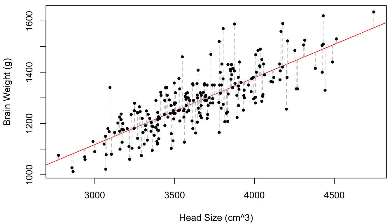

Figure 1.1: Brain weight vs. head size for 236 subjects. The line of best-fit is provided in red and the vertical distances between the points and the line (of which the sum-of-squares is minimized by the given line) are given in dotted grey.

While the size of the head can be measured on a live subject, the weight of the brain can only be calculated post-mortem by removing it from the skull. Therefore, it would be interesting to “predict” the brain weight of a live subject from observable characteristics – such as the size of the head.

This problem was first tackled over 200 years ago by French mathematician Adrien-Marie Legendre. Legendre’s formulation of the problem was:

Given a scatterplot of points \((x_1, y_1), (x_2, y_2), \ldots, (x_n, y_n)\), find the “best-fitting” line of the form \(y = \beta_0 + \beta_1 x\).

Legendre’s solution was to minimize the vertical distance between the straight line and each of the points, i.e., to minimize the sum-of-squares \[\begin{equation} S(\beta_0, \beta_1) = \sum_{i=1}^n (y_i - \beta_0 - \beta_1 x_i)^2. \tag{1.1} \end{equation}\] It is relatively straighforward to show (see Section 1.2.2) that the values of \(\beta_0\) and \(\beta_1\) which minimize (1.1) are \[\begin{equation} \hat \beta_1 = \frac{\sum_{i=1}^n(y_i - \bar y)(x_i - \bar x)}{\sum_{i=1}^n (x_i - \bar x)^2}, \qquad \hat \beta_0 = \bar y - \hat \beta_1 \bar x, \tag{1.2} \end{equation}\] where \(\bar x = \frac 1 n \sum_{i=1}^n x_i\) and \(\bar y = \frac 1 n \sum_{i=1}^n y_i\).

Legendre called his solution the least-squares method (Legendre (1805), p.45). While highly influential at the time (and still today!), Legendre’s method leaves several questions unanswered:

• Q1: Why do we minimize vertical distances? Why not horizontal distances, or better yet, the shortest (i.e., perpendicular) distance between the points and the line?

• Q2: According to Legendre’s formula, we have \(\hat \beta_0 = 335.43\) and \(\hat \beta_1 = 0.26\). Therefore, in some sense the “best prediction” for the brain mass of an individual with head size of \(x = 4000\)cm\(^3\) is \(y = 335.43 +0.26 \times 4000 = 1378.72\)g. However, Figure 1.1 clearly indicates that the \(y\) values near \(x = 4000\) are not all exactly equal to 1378.72. How can we account for this in our prediction?

• Q3: We would imagine that if measurements for a new set of 236 subjects were recorded, the least-squares estimates of \(\beta_0\) and \(\beta_1\) would probably be different. How large could this difference be? Is it possible that the estimated slope would actually be negative?

These questions can all be answered by a different treatment of the problem, published only four years after the work of Legendre, by the prince of mathematicians, Carl Friedrich Gauss. Gauss’ seminal insight was that, for a subject with head size equal to \(x_i\), the brain weight \(y_i\) is randomly drawn from the population of all individuals with head size \(x_i\). Thus, “predicting” \(y\) given \(x\) becomes the task of estimating the conditional distribution \(p(y \mid x)\). The model Gauss used for this conditional distribution, i.e., for generating \(y_i\) given \(x_i\), is \[\begin{equation} y_i = \beta_0 + \beta_1 x_i + \eps_i, \qquad \eps_i \iid \N(0,\sigma^2). \tag{1.3} \end{equation}\] In fact, it was for this very problem that Gauss invented the distribution which bears his name! Letting \(y = (\rv y n)\) and \(x = (\rv x n)\), (1.3) fully specifies the conditional distribution \(p(y \mid x, \beta_0, \beta_1, \sigma) = \prod_{i=1}^n p(y_i \mid x_i, \beta_0, \beta_1, \sigma)\). We will see momentarily that the log-likelihood function of the parameters \(\theta = (\beta_0, \beta_1, \sigma)\) is \[\begin{align*} \ell(\theta \mid y, x) & = - \frac 1 2 \frac{\sum_{i=1}^n (y_i - \beta_0 - \beta_1 x_i)^2}{\sigma^2} - \frac n 2 \log(\sigma^2) \\ & = - \frac 1 {2\sigma^2} S(\beta_0, \beta_1) - \frac n 2 \log(\sigma^2), \end{align*}\] such that for any value of \(\sigma > 0\), the values of \(\beta_0\) and \(\beta_1\) which maximize \(\ell(\theta \mid y, x)\) are precisely Legendre’s least-squares solution to (1.1). Thus, the statistical treatment of the problem pioneered by Gauss immediately produces an answer to above. We shall see that it also produces answers to and – and more! It is the fundamental tool for regression analysis, the statistical analysis of the relationships among variables from experimental data. In fact, a slight generalization of Gauss’ model (1.3) to several explanatory variables is \[\begin{equation} y_i = \beta_0 + \beta_1 x_{i1} + \cdots + \beta_p x_{ip} + \eps_i, \qquad \eps_i \iid \N(0, \sigma^2). \tag{1.4} \end{equation}\] This is the so-called multiple linear regression model. It is the main object of study in this course and perhaps the most versatile and widely-used statistical tool developed to date.

1.1.1 Notation and Review

In the following sections, we will derive the least-squares estimators \(\hat \beta_0\) and \(\hat \beta_1\) for the simple linear regression model (1.3) (simple = only one covariate). We’ll also state without proof the results that can be used to answer questions - above. The proofs will be derived formally when we cover the more general multiple linear regression model (1.4).

First, let’s go over some conventions I’ll be using throughout the class.

• \(Y, y, X, x\), etc. can all be random/nonrandom scalars/vectors. The right interpretation will be specified explicitly or unambiguously interpretable from the context.

• Most of the random variables in this class are continuous. Their pdf or conditional pdf will be denoted by e.g., \(f_Y(y)\) or \(f(y)\), and \(f_{Y\mid X}(y\mid x)\) or \(f(y\mid x)\). The notation \(p(y)\) or \(p(Y \mid X)\) means the distribution of \(y\), or the conditional distribution of \(Y\) given \(X\). The distribution of a random variable is an umbrella term for its pdf, cdf, pmf, or a name (e.g., normal, uniform). Any of these conveys the same information: everything we need to know to evaluate the probability statements \(\Pr(y \in A)\) and \(\Pr(Y \in A \mid X \in B)\). For example, if \(Y \mid X \sim \N(2X, 1)\), then \(\Pr(Y < 2 \mid X = 1) = \tfrac 1 2\).

Here is a quick review of some useful concepts:

• The mean of a continuous random variable \(Y\) with pdf \(f(y)\) is defined as \[ \E[Y] = \intii y f(y) \ud y. \] Recall the linearity of expectation: \[ \E\Big[\sumi 1 n a_i Y_i + b\Big] = \sumi 1 n a_i \E[Y_i] + b. \] Given \((\rv Y n)\), the sample mean is defined as \(\bar Y = \frac 1 n \sum_{i=1}^n Y_i\).

• The variance of \(Y\) is defined as \[ \var(Y) = \E[(Y - \E[Y])^2] = \E[Y^2] - (\E[Y])^2. \] Recall that \(\var(aY + b) = a^2 \var(Y)\), and that for independent random variables \(X \amalg Y\), \(\var(X+Y) = \var(X) + \var(Y)\). The sample variance is defined as \[ s_Y^2 = s_{YY} = \frac{S_{YY}}{n-1} = \frac 1 {n-1} \sum_{i=1}^n (Y_i - \bar Y)^2 = \frac{\sum_{i=1}^n Y_i^2 - n (\bar Y)^2}{n-1}. \]

• The covariance between two random variables \(X\) and \(Y\) is defined as \[ \cov(X, Y) = \E[(X-\E[X])(Y-\E[Y])] = \E[XY] - \E[X]\E[Y]. \] Note that \(\cov(X, X) = \var(X)\) and \(\cov(aX + c, bY + d) = ab\cdot\cov(X,Y)\). Moreover, for a collection of random variables \(\rv Y n\) we have \[ \cov\left(\sum_{i=1}^n a_i Y_i + c, \sum_{j=1}^n b_j Y_j + d\right) = \sum_{i=1}^n\sum_{j=1}^n a_ib_j \cov(Y_i, Y_j). \] In particular, this means that \[ \var\left(\sum_{i=1}^n a_i Y_i \right) = \sum_{i=1}^n a_i^2 \var(Y_i) + \sum_{i\neq j} a_ia_j \cov(Y_i, Y_j) \] The sample covariance is defined as \[ s_{XY} = \frac{S_{XY}}{n-1} = \frac 1 {n-1} \sum_{i=1}^n (X_i - \bar X)(Y_i - \bar Y) = \frac{\sum_{i=1}^n X_i Y_i - n \bar X \bar Y}{n-1}. \]

Finally, here are the main distributions we will be using in this class:

• If \(Z\) is has a normal distribution with mean \(\mu\) and variance \(\sigma^2\), this is denoted \(Z \sim \N(\mu, \sigma^2)\). The pdf of \(Z\) is \[ f(z) = \frac{1}{\sqrt{2\pi\sigma^2}} \exp\left\{- \frac{(z-\mu)^2}{2\sigma^2} \right\}. \] Recall that if \(Z_i \ind \N(\mu_i, \sigma_i^2)\), then \(W = \sum_{i=1}^n a_i Z_i + b\) is also normal: \[ W \sim \N\Big(\sum_{i=1}^n a_i\mu_i + b, \sum_{i=1}^n a_i^2 \sigma_i^2 \Big). \]

• If \(X\) has a chi-squared distribution with degrees-of-freedom parameter \(\nu\), this is denoted \(X \sim \chi^2_{(\nu)}\). The pdf of \(X > 0\) is \[ f(x) = \frac{1}{2^{\nu/2}\Gamma(\nu/2)} x^{\nu/2-1}e^{-x/2}. \] Recall that if \(\rv Z n \iid \N(0,1)\), then \(X = \sum_{i=1}^n Z_i^2 \sim \chi^2_{(n)}\). Moreover, the mean and variance of the chi-square are \(\E[X] = \nu\) and \(\var(X) = 2\nu\).

• If \(Y\) has a Student-\(\bm t\) (or simply \(t\)) distribution with degrees-of-freedom parameter \(\nu\), this is denoted \(Y \sim t_{(\nu)}\). The pdf of \(Y\) is \[ f(y) = \frac{\Gamma(\nu/2+\tfrac 1 2)}{\sqrt{\pi\nu} \Gamma(\nu/2)} \left(1 + \frac{y^2}{\nu}\right)^{-\frac{\nu+1}{2}}. \] Recall that if \(Z \sim \N(0,1)\), \(X \sim \chi^2_{(\nu)}\), and \(Z \amalg X\), then \(Y = Z/\sqrt{X/\nu} \sim t_{(\nu)}\). For the mean and of the \(t\)-distribution is \(\E[Y] = 0\), and for \(\nu > 2\), its variance is \(\var(Y) = \nu/(\nu - 2)\). For \(\nu < 2\), we have \(\var(Y) = \infty\).

1.2 Maximum Likelihood Estimation

1.2.1 Likelihood Function for the Linear Model

The statistical model (1.3) stipulated by Gauss implicitly makes the following assumptions:

• A1: The vector of covariates \(x = (\rv x n)\) are fixed and known.
• A2: The model parameters \(\theta = (\beta_0, \beta_1, \sigma)\) are fixed and unknown.
• A3: The vector of responses \(y = (\rv y n)\) are random.

Such a setup allows us to specify a probability distribution \(p(y \mid x, \theta)\) for the random quantities for any value of the fixed quantities, be they known or unknown. Under -, the following model formulation is equivalent to (1.3): \[\begin{equation} y_i \mid x_i \ind \N(\beta_0 + \beta_1 x_i, \sigma^2). \tag{1.5} \end{equation}\] Note that these three other model formulations are also equivalent to (1.3) under -: \[\begin{align} & y_i \mid x, \theta \ind \N(\beta_0 + \beta_1 x_i, \sigma^2), \tag{1.6} \\ & y_i \mid x \ind \N(\beta_0 + \beta_1 x_i, \sigma^2), \tag{1.7} \\ & y_i \ind \N(\beta_0 + \beta_1 x_i, \sigma^2) \tag{1.8}. \end{align}\] However, it is easy to imagine a situation where the covariates \(x\) are also random. For instance, if we randomly picked a new set of \(n = 236\) patients, we would most likely get a new set of head size measurements. When is relaxed such that the \(x_i\) are also random, then only (1.6) and (1.7) are equivalent to (1.3), whereas (1.5) and (1.8) are not.

The reason for which we assume that \(x\) are not random is in order to specify the likelihood function, \[ \mathcal L(\theta \mid \tx{data}) \propto p(\tx{data} \mid \theta). \] Strictly speaking, the data is \((y, x)\), such that \(\mathcal L(\theta \mid y, x) \propto p(y, x \mid \theta) = p(y \mid x, \theta) p(x \mid \theta)\). Thus, if \(x\) is random, we are forced to specify its probabilistic dependence on the model parameters. Pretending that \(x\) is fixed simply amounts to specifying that \(p(x \mid \theta) = p(x)\).

Upon assuming that \(x\) is fixed, we can use (1.5) to write down the likelihood function for \(\theta\): \[\begin{align*} \mathcal L(\theta \mid y, x) \propto p(y \mid x, \theta) & = \prod_{i=1}^n p(y_i \mid x_i, \theta) \\ & \propto \frac{1}{\sigma^n}\exp\left\{- \sum_{i=1}^n \frac {(y_i - \beta_0 - \beta_1 x_i)^2}{2\sigma^2} \right\}. \end{align*}\]

Notation: Throughout this course we will assume that - hold, unless explicitly stated otherwise. When this is the case, we’ll use (1.5) to designate the simple linear regression model. It’s the one most commonly used in textbooks and reminds us that (1.3) is a conditional probability model, without constantly dragging around the fixed value of \(\theta\). Since - hold, we can condition on \(x\), \(x_i\), and/or \(\theta\) whenever we want without changing the meaning of the equation. All that this does is draw our attention to a particular aspect of the model that we wish to emphasize.

1.2.2 Derivation of the MLE of \(\beta_0\) and \(\beta_1\)

Recall that since \(f(x_1) > f(x_2) \iff \log(f(x_1)) > \log(f(x_2))\), the value of \(x\) which maximizes \(f(x)\) also maximizes \(\log(f(x))\). Therefore, to find the maximum likelihood estimate of \(\theta\), we can instead maximize the log-likelihood \[ \ell(\theta \mid y, x) = \log(\mathcal L(\theta \mid y, x)) = -\frac 1 2 \left[n \log(\sigma^2) + \frac{\sum_{i=1}^n (y_i - \beta_0 - \beta_1 x_i)^2}{\sigma^2} \right]. \] It’s almost always easier to do the maximization on the log scale and there are other reasons for doing it this way as well (which we’ll hopefully see later). The MLE of \(\theta\) is obtained by setting the partial derivatives of the log-likelihood function to zero. \[\begin{align} \fdel {\beta_0}{\ell(\theta \mid y, x)} & = \frac 1 {\sigma^2} \sum_{i=1}^n (y_i - \beta_0 - \beta_1 x_i) = 0, \tag{1.9} \\ \fdel {\beta_1}{\ell(\theta \mid y, x)} & = \frac 1 {\sigma^2} \sum_{i=1}^n (y_i - \beta_0 - \beta_1 x_i)x_i = 0, \tag{1.10} \\ \fdel {\sigma^2}{\ell(\theta \mid y, x)} & = \frac{\sum_{i=1}^n (y_i - \beta_0 - \beta_1 x_i)^2}{2} \times \frac 1 {[\sigma^2]^2} - \frac n 2 \times \frac 1 {\sigma^2} = 0. \tag{1.11} \end{align}\] Multiplying both sides of (1.9) by \(\sigma^2/n\) and both sides of (1.10) by \(\sigma^2\) yields \[\begin{align*} \bar y - \beta_0 - \beta_1 \bar x & = 0, \\ \sum_{i=1}^n x_i y_i - n \beta_0 \bar x - \beta_1 \sum_{i=1}^n x_i^2 & = 0 \end{align*}\] such that \(\beta_0 = \bar y - \beta_1 \bar x\) from (1.9) and substituting this into (1.10) gives \[ \sum_{i=1}^n x_i y_i - n(\bar y - \beta_1 \bar x)\bar x - \beta_1 \sum_{i=1}^n x_i^2 = 0 \implies \beta_1 \left[\sum_{i=1}^n x_i^2 - n(\bar x)^2 \right] = \sum_{i=1}^n x_i y_i - n \bar x \bar y. \] Therefore, the maximum likelihood (ML) estimators of \(\beta_0\) and \(\beta_1\) are \[\begin{equation} \begin{split} \hat \beta_1\sp{ML} & = \frac{\sum_{i=1}^n(y_i - \bar y)(x_i - \bar x)}{\sum_{i=1}^n(x_i - \bar x)^2} = \frac{S_{yx}}{S_{xx}} = \frac{s_{yx}}{s_{xx}}, \\ \hat \beta_0\sp{ML} & = \bar y - \hat \beta_1\sp{ML} \bar x, \end{split} \tag{1.12} \end{equation}\] and these are exactly equal to the least-squares estimators \(\hat \beta_0\sp{LS}\) and \(\hat \beta_1\sp{LS}\) from (1.2).

Notation: From now on, we’ll denote the ML and LS estimates of \(\beta_0\) and \(\beta_1\) simply by \(\hat \beta_0\) and \(\hat \beta_1\), unless explictitly stated otherwise.

1.2.3 MLE vs. Unbiased Estimator of \(\sigma^2\)

To find \(\hat \sigma\sp{ML}\), we solve for the last equation (1.11). Let us first define the following terms: - \(\hat y_i = \hat \beta_0 + \hat \beta_1 x_i\) is called the \(i\)th predicted value. - \(e_i = y_i - \hat y_i\) is called the \(i\)th residual. If we plug \(\hat \beta_0\) and \(\hat \beta_1\) into (1.11) and multiply both sides of (1.11) by \([\sigma^2]^2/2\), we obtain \[ \sum_{i=1}^n e_i^2 - n \hat \sigma^2 = 0 \implies \hat\sigma^{2(ML)} = \frac{\sum_{i=1}^ne_i^2}{n}. \] Thus, \[\begin{align*} \max_\theta \ell(\theta \mid y, x) & = -\frac 1 2 \left[n \log(\sigma^{2(ML)}) + \frac{\sum_{i=1}^n (y_i - \hat\beta_0 - \hat\beta_1 x_i)^2}{\hat\sigma^{2(ML)}} \right] \\ & = -\frac 1 2 \left[n \log(s^2) + \frac{\sum_{i=1}^n (y_i - \hat\beta_0 - \hat\beta_1 x_i)^2}{s^2} \right], \end{align*}\] where \(s = \sqrt{\hat \sigma^{2(ML)}}\). In other words, the maximum possible value of the log-likelihood is obtained when \(s = \sqrt{\hat \sigma^{2(ML)}}\) is plugged in for \(\sigma\), such that the MLE of \(\sigma\) is \(\hat \sigma^{(ML)} = \sqrt{\hat \sigma^{2(ML)}}\).

However, a different estimator of \(\sigma\) is commonly used, namely: \[ \hat \sigma^2 = \frac{\sum_{i=1}^n e_i^2}{n-2}. \] The reason for this is that a scaled version of \(\sum_{i=1}^n e_i^2\) has a chi-squared distribution: \[\begin{equation} \frac{1}{\sigma^2} \sum_{i=1}^n e_i^2 \sim \chi^2_{(n-2)}. \tag{1.13} \end{equation}\] Recall that the expectation of a \(\chi^2_{(\nu)}\) is \(\nu\), such that \(\E[\hat \sigma^2 \mid \theta] = \sigma^2\), regardless of the true value of \(\theta\). In other words, \(\hat \sigma^2\) is an unbiased estimator of \(\sigma^2\).

The difference between \(\hat \sigma\) and \(\hat \sigma\sp{ML}\) is usually inconsequential: for \(n \ge 50\) is is less than 2%. However, \(\hat \sigma\) is automatically reported by \(\R\) and using it instead of \(\hat \sigma\sp{ML}\) makes the upcoming formulas slightly simpler. For this reason we’ll use it to estimate \(\sigma\) from now on, unless explicitly stated otherwise.

Example 1.1 The estimates of \(\hat \beta_1\), \(\hat \beta_0\), and \(\hat \sigma\) for Dr. Gladstone’s data can be calculated in \(\R\) as follows:

# load the brain data into R
brain <- read.csv(file = "brainhead.csv")
head(brain)

##   gender   age head.size brain.wgt
## 1      M 20-46      4512      1530
## 2      M 20-46      3738      1297
## 3      M 20-46      4261      1335
## 4      M 20-46      3777      1282
## 5      M 20-46      4177      1590
## 6      M 20-46      3585      1300

# assign the columns to variable names
x <- brain$head.size # head size
y <- brain$brain.wgt # brain weight

b1.hat <- cov(x,y)/var(x) # cov(x,y) = s_{xy}, var(x) = s_{xx}
b0.hat <- mean(y) - mean(x) * b1.hat # mean(y) = y.bar
y.hat <- b0.hat + b1.hat * x # predicted values
res <- y - y.hat # residuals
n <- length(y) # number of observations
# res^2 squares each residual without using a for-loop
sigma.hat <- sqrt(sum(res^2)/(n-2))

# display nicely
signif(c(b1.hat = b1.hat, b0.hat = b0.hat, sigma.hat = sigma.hat), 2)

##    b1.hat    b0.hat sigma.hat 
##      0.26    340.00     72.00

In fact, a simpler \(\R\) way of calculating the MLEs of \((\beta_0,\beta_1)\) is with the command:

M <- lm(y ~ x) # fit linear model
signif(coef(M), digits = 2) # MLE's of beta

## (Intercept)           x 
##      340.00        0.26

Note the syntax of the command, which automatically assumes an intercept term.

1.3 Interval Estimates of \(\beta_0\) and \(\beta_1\)

Notice that for fixed (i.e., nonrandom) values of \(x\) (as in ), we can rewrite \(\hat \beta_1\) as a linear combination of the \(y_i\): \[ \hat \beta_1 = \frac{\sum_{i=1}^n(y_i - \bar y)(x_i - \bar x)}{\sum_{i=1}^n(x_i - \bar x)^2} = \sum_{i=1}^n w_i(y_i - \bar y) = \sum_{i=1}^n w_i y_i - n \bar w \bar y = \sum_{i=1}^n (w_i - \bar w) y_i, \] where \(w_i = (x_i-\bar x)/\sum_{i=1}^n(x_i-\bar x)^2\). Using (1.5) and the additive property of independent normals, we have \[\begin{align*} \hat \beta_1 & \sim \N\left(\sum_{i=1}^n(w_i - \bar w)(\beta_0 + \beta_1 x_i), \sigma^2 \sum_{i=1}^n (w_i - \bar w)^2 \right) \\ & \sim \N\left(\beta_1, \sigma^2 \times \frac{1}{S_{xx}}\right). \end{align*}\]

1.3.1 Treatment for Known \(\sigma\)

If the value of \(\sigma\) were known, then we could just use \(\sigma_1 = \sigma/\sqrt{S_{xx}}\) to create a 95% confidence interval for \(\beta_1\), since \(Z = (\beta_1 - \hat \beta_1)/\sigma_1 \sim \N(0,1)\), such that \[\begin{align*} 95% & = \Pr(-1.96 < Z < 1.96 \mid \theta) \\ & = \Pr(-1.96 < (\beta_1 - \hat \beta_1)/\sigma_1 < 1.96 \mid \theta) \\ & = \Pr(-1.96 \sigma_1 < \beta_1 - \hat \beta_1 < 1.96 \sigma_1 \mid \theta) \\ & = \Pr(\hat \beta_1 - 1.96 \sigma_1 < \beta_1 < \hat \beta_1 + 1.96 \sigma_1 \mid \theta). \end{align*}\] Thus, if we repeat the experiment over and over again, the interval \(\hat \beta_1 \pm 1.96 \sigma_1\) will have a 95% chance of covering the true value of \(\beta_1\), regardless of the true value of the parameters \(\theta = (\beta_0, \beta_1, \sigma)\).

1.3.2 Treatment for Unknown \(\sigma\)

In practice, however, the true value of \(\sigma\) is typically unknown, so \(\sigma_1\) is unavailable to us. Instead, we turn to the unbiased estimator \(\hat \sigma^2 = \frac{1}{n-2} \sum_{i=1}^n e_i^2\). We have already seen that \[ \frac{1}{\sigma^2} \sum_{i=1}^n e_i^2 = (n-2)/\sigma^2 \cdot \hat \sigma^2 \sim \chi^2_{(n-2)}. \] Moreover, it turns out that \(\hat \sigma^2\) is independent of \(\hat \beta_0\) and \(\hat \beta_1\). Therefore, since \(Z = (\beta_1 - \hat \beta_1)/\sigma_1 \sim \N(0,1)\) and independently \(X = (n-2)/\sigma^2 \times \hat \sigma^2 \sim \chi^2_{(n-2)}\), \[ Y = \frac{Z}{\sqrt{\frac{X}{n-2}}} = \frac{\beta_1 - \hat \beta_1}{s_1} \sim t_{(n-2)}, \where s_1 = \hat \sigma/\sqrt{S_{xx}}. \] Note that \(Y \sim t_{(n-2)}\) for any value of \(\theta\). Therefore, we can build a \((1-\alpha)\)-level confidence interval for \(\beta_1\) as follows.

1. Find \(q\) such that \(\Pr(-q < Y < q) = 1-\alpha\). To do this, note that \(Y \sim t_{(n-2)}\) is symmetric, and therefore \[ 1-\alpha = \Pr(-q < Y < q) = 1 - \Pr(\abs{ Y } > q) = 1 - 2\Pr(Y < -q) \implies \Pr(Y < -q) = \alpha/2. \] In other words, \(q\) can be obtained by inverting the CDF of \(Y\). In \(\R\) this is done with the command:

   conf <- .95 # for a 95% confidence interval
   alpha <- 1-conf
   q <- -qt(p = alpha/2, df = n-2)

2. Once the correct “quantile” q has been found, the procedure is identical as when \(\sigma\) is known, upon replacing \(\sigma_1\) by \(s_1\): \[\begin{align*} 1-\alpha & = \Pr(-q < Y < q \mid \theta) \\ & = \Pr(-q < (\beta_1 - \hat \beta_1)/s_1 < q \mid \theta) \\ & = \Pr(\hat \beta_1 - q s_1 < \beta_1 < \hat \beta_1 + q s_1 \mid \theta). \end{align*}\]

Thus, \(\hat \beta_1 \pm q s_1\) is a \((1-\alpha)\) confidence interval for \(\beta_1\) which can be used when the entire parameter vector \(\theta = (\beta_0, \beta_1, \sigma)\) is unknown.

Example 1.2 For the brain weight data, we have \(n = 236\) and \[\begin{align*} \bar x & = 3637.86, & \bar y & = 1284.26, \\ s_{xx} & = 130413.76, & s_{xy} & = 34014.61, & \hat \sigma^2 & = 5234.62. \end{align*}\] For a 95% confidence interval, we calculate \(q = 1.97\). Compare this to the 95% value for a \(\N(0,1)\), which is 1.96. Moreover, \[ s_1 = \hat \sigma/\sqrt{S_{xx}} = \hat \sigma /\sqrt{(n-1)s_{xx}} = \sqrt{\frac{5234.62}{235\times130413.76}} = 0.01. \] The confidence interval for \(\beta_1\) is thus \[ \hat \beta_1 \pm 1.97 \times s_1 = (0.24, 0.29). \]

Question: Does this mean that there is a 95% probability of finding \(\beta_1\) between 0.24 and 0.29?

Remark. The construction of a confidence interval for \(\beta_0\) is completely analogous:

1. Start by writing \(\hat \beta_0 = \bar y - \hat \beta_1 \bar x\) as a linear combination of the \(y_i\), and upon simplification find that

   \[ \hat \beta_0 = \sim \N\left(\beta_0, \sigma^2 \times \left[\frac 1 n + \frac{\bar{x}^2}{S_{xx}}\right]\right). \]

2. Assume that \(\hat \beta_0\) and \(\hat \sigma\) are independent random variables (which we’ll prove later in the course). Then upon defining \(s_0 = \hat \sigma \sqrt{1/n + \bar x^2/S_{xx}}\), we have

   \[ Y = \frac{\beta_0 - \hat \beta_0}{s_0} \sim t_{(n-2)} \]

   for any value of \(\theta\).

3. Proceed exactly as for \(\beta_1\) to find \(q\) such that \(\Pr(\abs{ Y } < q) = 1-\alpha\), and then \(\hat \beta_0 \pm q s_0\) is a \((1-\alpha)\)-level confidence interval for \(\beta_0\).

1.4 Hypothesis Testing

A variant on the confidence interval procedure above can be used to answer . We shall first consider the more standard problem of assessing whether or not \(\beta_1 = 0\) in the classical framework of hypothesis testing. For a general statistical model of the form \(Y \sim p(Y \mid \theta)\), this framework proceeds as follows.

1. The first step is to establish a formal null hypothesis, \[ H_0: \theta = \theta_0, \]
2. Next, we look at the data \(Y\) and decide how we would quantify evidence against \(H_0\). Usually, this means look for some test statistic \(T = T(Y)\) such that extreme values of \(T\) (very low, very high, or both) would be unlikely if \(H_0\) were true.
3. If we are lucky, then \(T\) has a well-defined statistical distribution under \(H_0\): \[ T \sim p(T \mid H_0). \] Then if \(T_\obs = T(Y_\obs)\) is the particular value of the test statistic calculated for our dataset \(Y_\obs\), then \[\begin{equation} \Pr(T > T_\obs \mid H_0) \tag{1.14} \end{equation}\] is the probability that a new, randomly selected dataset \(Y\) will have a more extreme value of the test statistic than the one calculated for \(Y_\obs\). For example, if \(\Pr(T > T_\obs \mid H_0) = 0.1%\), then if \(H_0\) is true, only 1 in 1000 datasets will give more evidence against \(H_0\) than \(Y_\obs\).

The probability (1.14) is called a \(p\)-value. It is a quantitative measure of the evidence we have against \(H_0\). If we need to make an accept/reject decision about the null hypothesis, one way is to set a “cutoff” \(p\)-value – often 5%. If the calculated \(p\)-value is below 5%, then we decided that the observed value of the test statistic \(T_\obs\) is sufficiently “rare”. Indeed, if we reject \(H_0\) whenever we get a \(p\)-value below 5%, then if \(H_0\) is true and we repeat the experiment over and over then we will only reject \(H_0\) incorrectly 5% of the time. This is called the Type-I error.

In the context of our simple linear regression problem, the null hypothesis is \(H_0: \beta_1 = 0\). A natural choice of test statistic is \(\hat \beta_1 = \hat \beta_1(y, x)\), for which large positive or negative values constitute evidence against \(H_0\). To calculate the \(p\)-value for a given problem, we would need \(p(\hat \beta_1 \mid H_0)\). Unfortunately, \(H_0: \beta_1 = 0\) is not sufficient to specify this distribution, since \[ \hat \beta_1 \mid H_0 \sim \N\left(0, \sigma^2 \times \frac 1 {S_{xx}}\right). \] Therefore, the unknown value of \(\sigma\) is required to calculate the \(p\)-value of \(T_\obs = \hat \beta_1\).

Instead, let us consider a very general test statistic against \(H_0: \theta = \theta_0\) known as the likelihood ratio statistic: \[ \Lambda = T(Y) = \frac{\mathcal{L}(\hat \theta\sp{ML} \mid Y)}{\mathcal L(\theta_0 \mid Y)}. \] Since \(\max_\theta \mathcal L(\theta \mid Y) = \mathcal{L}(\hat \theta\sp{ML} \mid Y)\), we have \(\Lambda \ge 1\), and the larger the value of \(\Lambda\), the more likely that some other parameter \(\theta_1 \neq \theta_0\) is the true parameter values \(\theta = \theta_1\). Amazingly, the likelihood ratio statistic \(\Lambda\) for linear regression is equivalent to using the test statistic \(T = \hat \beta_1/s_1\), in the sense that \[ \Pr(\Lambda > \Lambda_\obs \mid \beta_1 = 0) = \Pr(\abs{ T } > \abs{ T_\obs } \mid \beta_1 = 0). \] Indeed, the distribution of \(T = \hat \beta_1/s_1\) is fully specified under the null \(H_0: \beta_1 = 0\): \[ \frac{\hat \beta_1}{s_1} \mid H_0 \sim t_{n-2}. \]

Example 1.3 For the brain weight dataset, we have \(\hat \beta_1 = 0.26\) and \(s_1 = 0.01\), such that \(T_\obs = \hat \beta_1/s_1 = 19.96\). To calculate the \(p\)-value against \(H_0: \beta_1= 0\), note that since \(T \mid H_0 \sim t_{(n-2)}\) is a symmetric distribution, we have \[ \Pr(\abs{ T } > \abs{ T_\obs }) = 2 \cdot \Pr(T > \abs{ T_\obs }) = 2 \cdot \Pr(T < -\abs{ T_\obs }). \] In \(\R\) we can calculate the \(p\)-value as follows:

T <- b1.hat/s1 # test statistic
pval <- 2*pt(q = -abs(T), df = n-2) # pvalue
pval

## [1] 2.031713e-52

So the calculated \(p\)-value is 0.00, which, for all practical purposes, is impossibly unlikely if \(H_0\) were true. So there is no way that under \(H_0\), we could randomly pick a sample of patients which would contain more evidence against \(H_0\). Thus, the given brain data produces considerable evidence against the absence of a relation between brain weight and head size.

1.5 Statistical Predictions

In addition to quantifying the degree of uncertainty about \(\hat \beta_1\), intervals estimates can be constructed to answer posed above. That is, suppose that we collect data \(y = (\rv y n)\) and \(x = (\rv x n)\). Now, for a new value of the covariate \(x_\star\), we wish to make a statement about its associated response, \(y_\star = y(x_\star) = \beta_\star + \beta_1 x_\star + \eps_\star\). To do this: 1. Consider the estimator \[ \hat y_\star = g(y, x, x_\star) = \hat \beta_0 + \hat \beta_1 x_\star \mid x_\star, x \sim \N\left(\beta_0 + \beta_1 x_\star, \sigma^2 \times \left[\frac 1 n + \frac {(x_\star-\bar x)^2} {S_{xx}} \right] \right). \] 2. Based on the data \(y = (\rv y n)\), a prediction interval for the random quantity \(y(x_\star)\) is a pair of random variables \(L = L(y,x,x_\star)\) and \(U = U(y,x,x_\star)\) such that \[ \Pr(L < y_\star < U \mid \theta) = 95%. \] 3. The difference here is that the middle quantity is now also random. However, since \(\hat y_\star = g(y, x, x_\star)\) and \(y_\star\) are independent random variables, we have \[\begin{equation} \hat y_\star - y_\star \mid x_\star, x \sim \N\left(0, \sigma^2 \times \left[1 + \frac 1 n + \frac {(x_\star-\bar x)^2} {S_{xx}} \right]\right). \tag{1.15} \end{equation}\] Therefore, a prediction interval for \(y_\star\) is based on \[ \frac{\hat y_\star - y_\star}{s(x_\star)} \sim t_{(n-2)}, \where s^2(x_\star) = \hat \sigma^2 \times \left[1 + \frac 1 n + \frac {(x_\star-\bar x)^2} {S_{xx}} \right]. \]

Example 1.4 For the brain weight data, Figure 1.2 displays the 95% confidence intervals about the line of best fit \(y(x) = \hat \beta_0 + \hat \beta_1 x\).

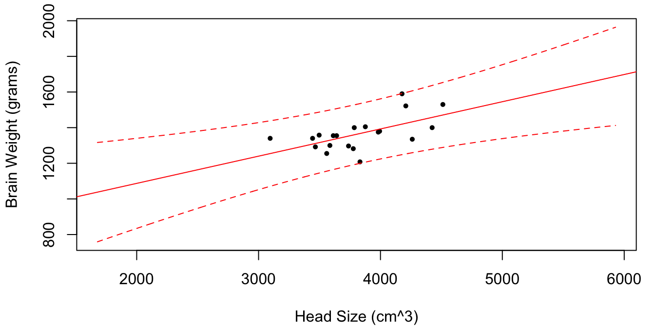
Figure 1.2: Brain weight vs. head size for \(n = 20\) randomly selected subjects. For each value of \(x\) in the plotting range the estimator \(\hat y(x) = \hat \beta_0 + \hat \beta_1 x\) is plotted in red, along with dotted lines for the 95% confidence intervals for the random quantity \(y(x)\). As \(x\) gets further and further from \(\bar x\), the size of the confidence interval increases.

For illustrative purposes, only \(n = 20\) patients were used to estimate \(\theta = (\beta_0, \beta_1, \sigma)\). We see that the closer the value of \(x_\star\) to the sample mean \(\bar x\), the smaller the confidence interval for \(y(x_\star)\). However, even as \(n \to \infty\), \(s(x_\star) \to \sigma\). This makes sense because \(\sigma\) is the intrinsic variability of the brain mass about their mean for a given value of head size. It is a population dependent parameter and does not decrease to 0. Thus, the confidence interval contains both a component due to population variability and a component due to estimation uncertainty.

As \(x_\star\) gets further and further from \(\bar x\), \(s(x_\star) \to \infty\). This is because a tiny change in the slope estimate \(\hat \beta_1\) has very large consequences far away from \(\bar x\). It also makes “intuitive sense” that out-of-sample predictions should be less and less certain the further the new data point is from data we have previously observed, as more extrapolation to make these predictions is required.

1.6 Checking the Modeling Assumptions

One of the truly beautiful aspects of the linear regression model (with normal errors) is that there are several ways to check whether the modeling assumptions are being violated. In particular, in addition to - which we assume for any conditional model \(p(y \mid x, \theta)\), the assumptions for the linear regression model (1.5) are:

• A4: The conditional mean of the response \(y_i\) is a linear function: \(\E[y_i \mid x_i] = \beta_0 + \beta_1 x_i\).
• A5: The conditional variance of \(y_i\) is constant: \(\var(y_i \mid x_i) = \sigma^2\).
• A6: The errors \(\eps_i = y_i - \beta_0 - \beta_1 x_i\) are iid normal: \(\eps_i \iid \N(0, \sigma^2)\).

One approach to model checking is to formulate it in a hypothesis testing framework: \[ H_0: y_i \mid x_i \ind \N(\beta_0 + \beta_1 x_i, \sigma^2), \tx{for some value of $\theta = (\beta_0, \beta_1, \theta)$}. \] In this case, the test statistics are typically based on the “standardized” model residuals: \[\begin{equation} z_i = \frac{e_i}{\hat \sigma} = \frac{y_i - \hat \beta_0 - \hat \beta_1 x_i}{\hat \sigma}. \tag{1.16} \end{equation}\] We shall cover this in more detail later, but for reasonably large \(n\) (I wouldn’t worry about any \(n \ge 100\)), it turns out that \[ z_i \mid H_0 \stackrel{\tx{iid}}{\approx} \N(0, 1). \] Based on these residuals, two of the most commonly used graphical devices for checking various aspects of - are:

1. The scatterplot of residuals vs. fitted values, \(e_i\) vs. \(\hat y_i = \hat \beta_0 + \hat \beta_1 x_i\).
2. A histogram or QQ-plot of the standardized residuals \(z_i\).

The following examples illustrate how these plots can be used to check assumptions -.

Example 1.5 (Nonlinear conditional mean) Consider synthetic data generated from the regression model (1.5) as follows:

n <- 500 # sample size
x <- rnorm(n) # predictors
eps <- rnorm(n) # errors

# model 1: E[y | x] is linear in x
y1 <- 1 + x + eps

That is, the true regression parameters are \(\beta_0 = \beta_1 = \sigma = 1\). Let’s use this data as a benchmark against data from which the mean is not linear in \(x\):

# model 2: E[y | x] is not linear in x
y2 <- 1 + (1+x)^2 + eps

For this second model, we have \(\E[y \mid x] = 1 + (1+x)^2\). The plots in Figure 1.3 display the scatterplots of the data from each model along with the line of best fit.

# fit linear models
M1 <- lm(y1 ~ x)
M2 <- lm(y2 ~ x)
# scatterplots of data with line of best fit
par(mfrow = c(1,2), mar = c(4,4,4,0)+.1)
pt.cex <- .7
plot(x, y1, pch = 16, cex = pt.cex,
     xlab = "x", ylab = "y", main = "Model 1")
abline(M1, col = "red")
plot(x, y2, pch = 16, cex = pt.cex,
     xlab = "x", ylab = "y", main = "Model 2")
abline(M2, col = "red")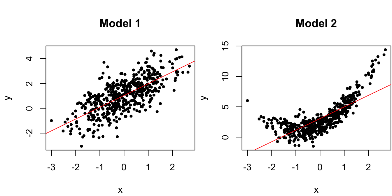

Figure 1.3: Scatterplots of data from the true regression model and a model with nonlinear mean.

We can clearly see here that the data from Model 2 violates the linear mean assumption , and such scatterplots are an extremely effective method of checking model assumptions for simple linear regression, i.e., with a single predictor \(x\). However, it is more difficult to construct scatterplots for multiple linear regression when there are several predictors, and thus residual vs. fitted value plots as in Figure 1.4 are used instead.

# residual vs fitted values
par(mfrow = c(1,2), mar = c(4,4,4,0)+.1)
pt.cex <- .7
plot(x = predict(M1), y = residuals(M1), # R way of calculating these
     pch = 16, cex = pt.cex,
     xlab = "Fitted Values", ylab = "Residuals", main = "Model 1")
abline(h = 0, col = "red", lty = 2) # add horizontal line
plot(x = predict(M2), y = residuals(M2),
     pch = 16, cex = pt.cex,
     xlab = "Fitted Values", ylab = "Residuals", main = "Model 2")
abline(h = 0, col = "red", lty = 2)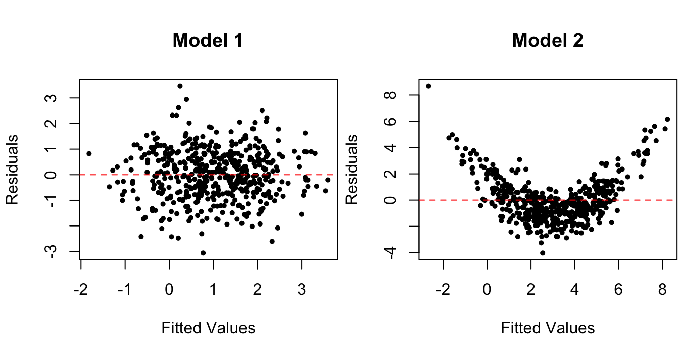

Figure 1.4: Residuals vs. fitted values for data from the true regression model and for one with nonlinear mean.

A horizontal line at zero is added to the plots. Indeed, the mean residual value is \[\begin{align*} \bar e = \frac 1 n \sumi 1 n e_i & = \frac 1 n \sumi 1 n(y_i - \hat \beta_0 - \hat \beta_1 x_i) \\ & = \bar y - \hat \beta_0 - \hat \beta_1 \bar x \\ & = -\hat \beta_0 + (\bar y - \hat \beta_1\bar x) = -\hat \beta_0 + \hat \beta_0 = 0. \end{align*}\] The nonlinearity of the mean is clearly visible for Model 2, in the right panel of Figure 1.4.

One thing to note is the “football shape” of the residuals in the left panel, under the true linear regression Model 1. That is, there appears to be less spread in the residuals for large/small fitted values \(\hat y_i\) than for values in the middle. This, however, is an artifact of there being more \(x_i\)’s near \(\bar x\) than far from it. Since we observe more residuals \(e_i\) in that area, we expect the range of the \(e_i\)’s to be larger in that area, even if assumptions - are correct.

Example 1.6 (Non-constant conditional variance) Let us keep the same synthetic data from the correct linear regression Model 1, but now generate responses with non-constant variance:

# Model 3: var(y | x) is not constant
y3 <- 1 + x + exp(x/3)*eps
# scatterplots and line of best fit
M3 <- lm(y3 ~ x)
par(mfrow = c(1,2), mar = c(4,4,4,0)+.1)
pt.cex <- .7
plot(x, y1, pch = 16, cex = pt.cex,
     xlab = "x", ylab = "y", main = "Model 1")
abline(M1, col = "red")
plot(x, y3, pch = 16, cex = pt.cex,
     xlab = "x", ylab = "y", main = "Model 3")
abline(M3, col = "red")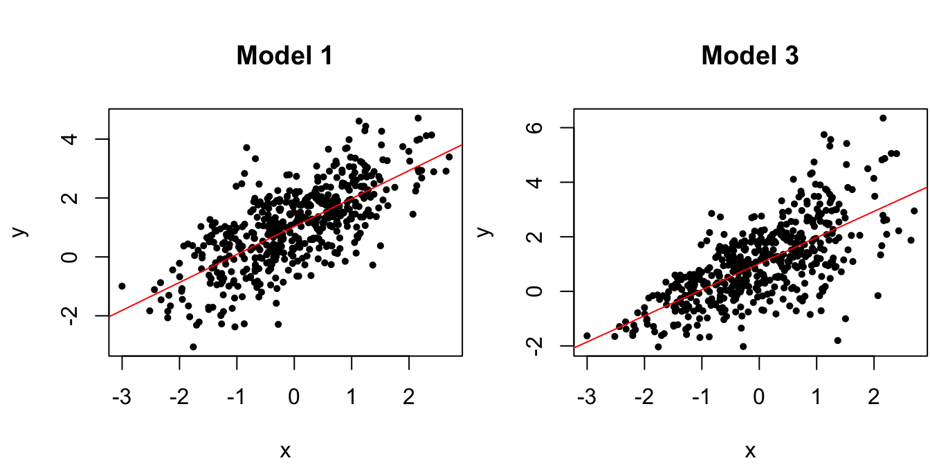

Figure 1.5: Scatterplots of data from the true regression model and a model with non-constant variance.

Once again, the violation of the constant conditional variance assumption is easy to spot from the scatterplot in Figure 1.5 when there is only one predictor, but such scatterplots do not reveal the information as clearly when there are multiple predictors. For this reason, one typically looks at the residual vs. fitted values instead:

# residual vs fitted values
par(mfrow = c(1,2), mar = c(4,4,4,0)+.1)
pt.cex <- .7
plot(x = predict(M1), y = residuals(M1), # R way of calculating these
     pch = 16, cex = pt.cex,
     xlab = "Fitted Values", ylab = "Residuals", main = "Model 1")
abline(h = 0, col = "red", lty = 2) # add horizontal line
plot(x = predict(M3), y = residuals(M3),
     pch = 16, cex = pt.cex,
     xlab = "Fitted Values", ylab = "Residuals", main = "Model 3")
abline(h = 0, col = "red", lty = 2)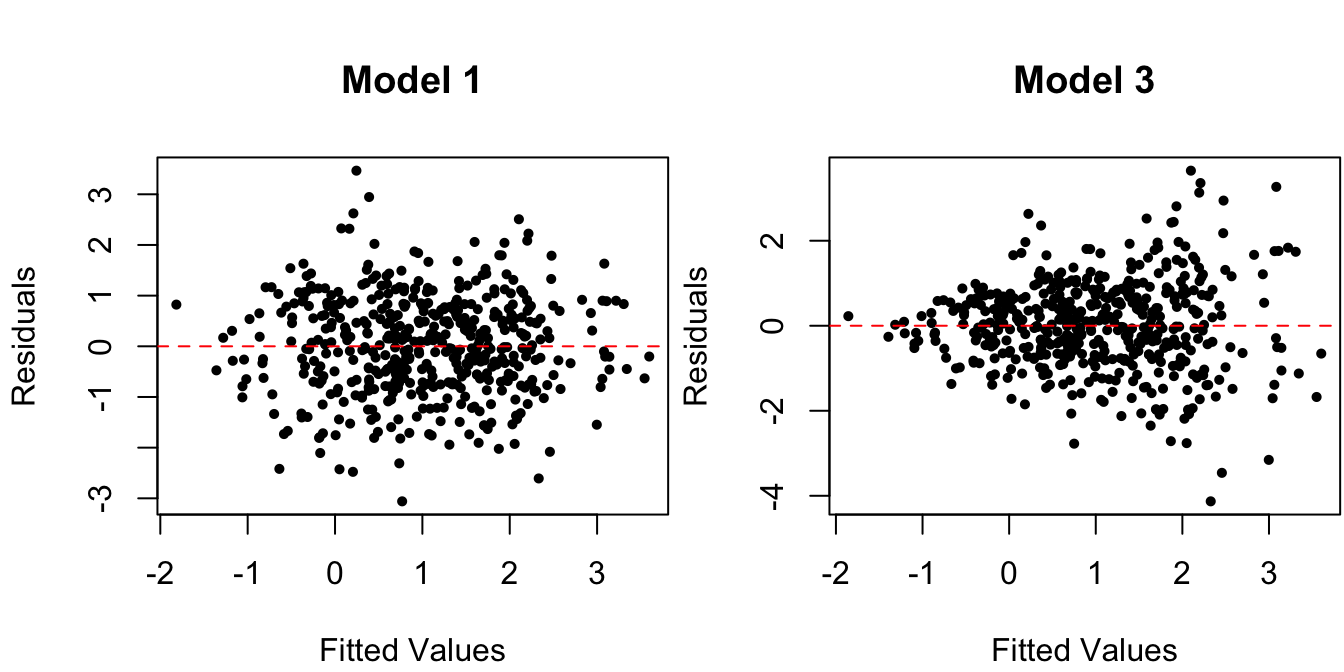

Figure 1.6: Residuals vs. fitted values for data from the true regression model and for one with non-constant variance.

Figure 1.6 displays a pattern of variance with the fitted value \(\hat y_i\), which is one of the most common patterns of non-constant variance (which we’ll cover later).

Example 1.7 (Non-normal errors) Again consider the synthetic data from the true regression Model 1, but now let’s compare it to data generated with non-normal errors:

# Model 4: errors are not normal
zeta <- rt(n, df = 3) # errors are t_(3)
y4 <- 1 + x + zeta
# residuals vs fitted values
M4 <- lm(y4 ~ x)
# residual vs fitted values
par(mfrow = c(1,2), mar = c(4,4,4,0)+.1)
pt.cex <- .7
plot(x = predict(M1), y = residuals(M1), # R way of calculating these
     pch = 16, cex = pt.cex,
     xlab = "Fitted Values", ylab = "Residuals", main = "Model 1")
abline(h = 0, col = "red", lty = 2) # add horizontal line
plot(x = predict(M4), y = residuals(M4),
     pch = 16, cex = pt.cex,
     xlab = "Fitted Values", ylab = "Residuals", main = "Model 4")
abline(h = 0, col = "red", lty = 2)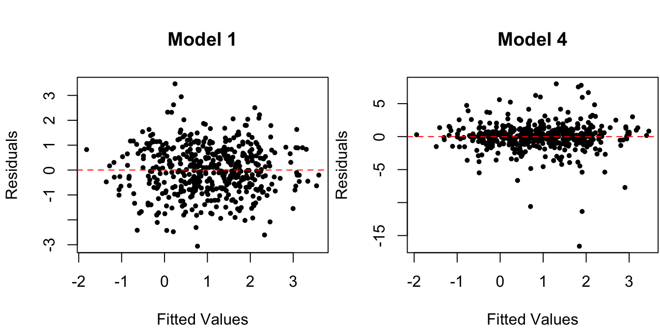

Figure 1.7: Residuals vs. fitted values for data from true regression model and one with non-normal (\(t_{(3)})\) distributed) errors.

The errors in Model 4 are drawn from a \(t_{(3)}\) distribution. However, the residuals vs. fitted value plots in Figure 1.7 do not reveal this violation of assumption . This is where the histograms and QQ-plots of the standardized residuals come in:

# calculate the standardized residuals
# Model 1
sig.hat1 <- sqrt(sum(residuals(M1)^2)/(n-2)) # sigma.hat
zres1 <- residuals(M1)/sig.hat1 # standardized residuals
# Model 4
sig.hat4 <- sqrt(sum(residuals(M4)^2)/(n-2))
zres4 <- residuals(M4)/sig.hat4

par(mfrow = c(2,2), mar = c(4,4,1,0)+.1)
# histograms
nbr <- 40
# Model 1
hist(zres1,
     breaks = nbr, # number of bins
     freq = FALSE, # make area under hist = 1 (as opposed to counts)
     xlab = "Standardized Residuals", main = "Model 1")
# add a standard normal curve for reference
curve(dnorm, add = TRUE, col = "red")
# same for Model 4
hist(zres4,
     breaks = nbr, freq = FALSE,
     xlab = "Standardized Residuals", main = "Model 4")
curve(dnorm, add = TRUE, col = "red")
# QQ-plots
# Model 1
qqnorm(zres1, main = "Model 1", pch = 16, cex = .7)
qqline(zres1, col = "red", lty = 2)
# Model 4
qqnorm(zres4, main = "Model 4", pch = 16, cex = .7)
qqline(zres4, col = "red", lty = 2)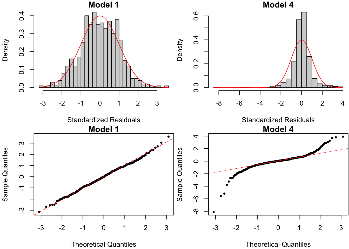

Figure 1.8: Histograms (top) and QQ-plots (bottom) of standardizeed residuals for data from true regression model and one with non-normal errors.

Both histograms and QQ-plots in Figure 1.8 attempt to uncover violations of the residuals’ normality assumption under \(H_0\). In this case, the presence of standardized residuals in Model 4 way out in the tail of their \(\N(0,1)\) distribution under \(H_0\) indicates that the error in Model 4 are heavy-tailed. A few more remarks: - Whether you plot the “raw” residuals \(e_i\) or the standardized residuals \(z_i = e_i/\hat \sigma\) is largely a matter of choice. The advantage of the former is that it is in unit of the original data (i.e., grams for brain weight). The advantage of the latter is that it is in units of standard deviations (i.e., 3 standard deviations from the mean is out in the 99% tail). - I find the histogram slightly easier to interpret, but visual conclusions depend very much on the number of bins used in the plot. On the other hand, the QQ-plot for a given set of residuals is unique. - In order to interpret residual plots, a few common non-normality patterns are illustrated in Figure 1.9.

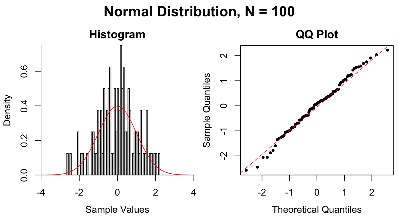
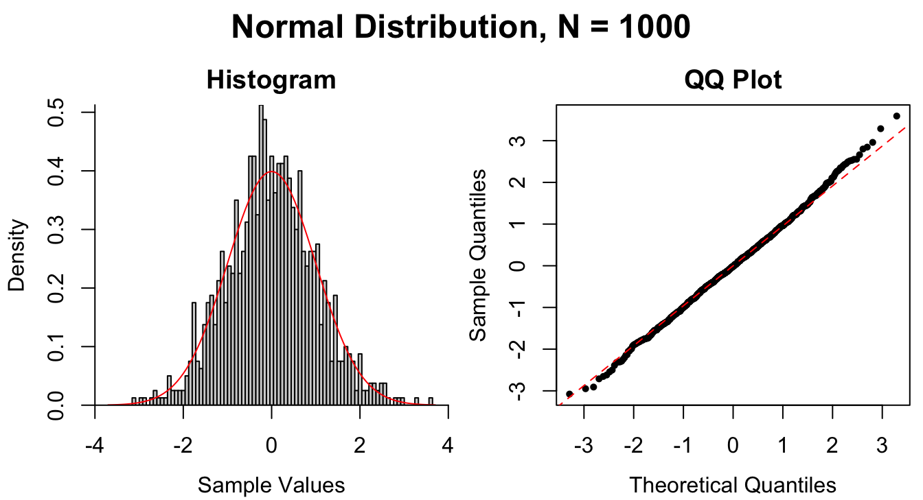
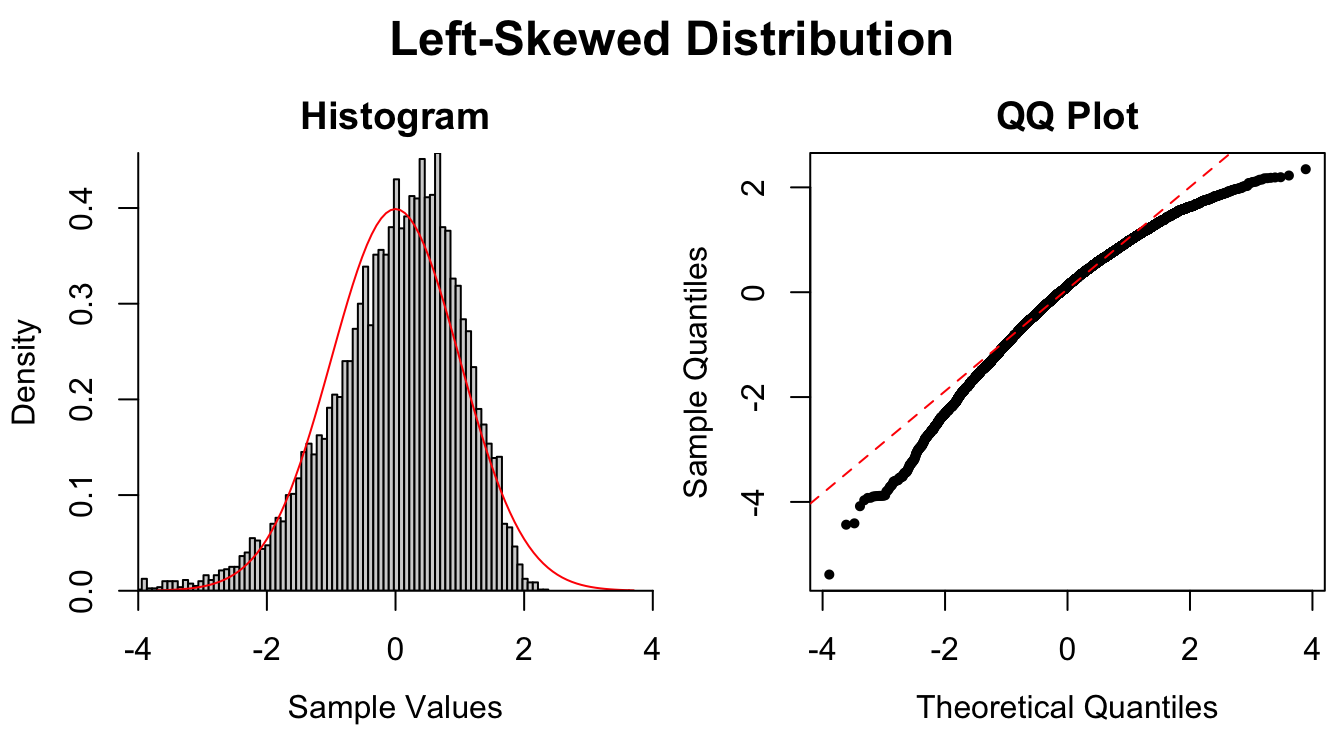
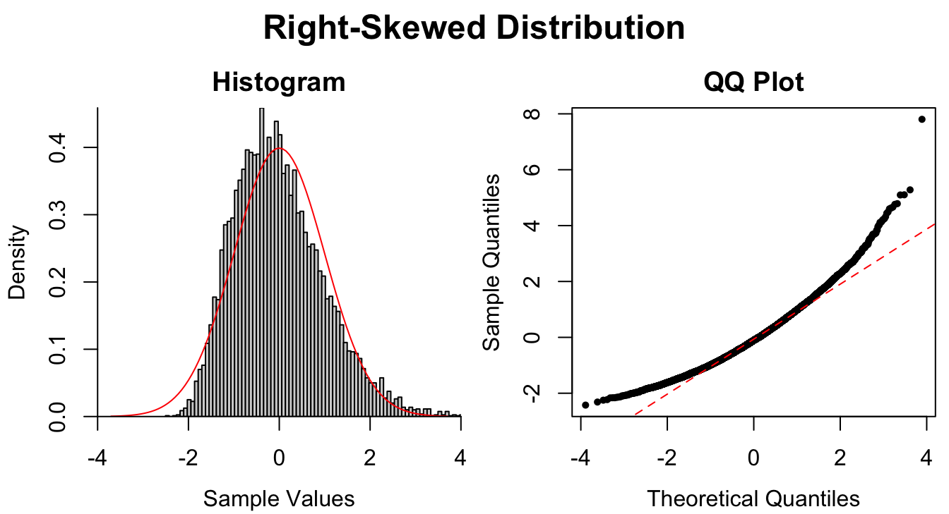
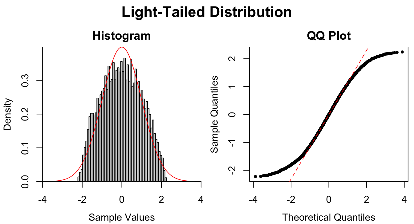
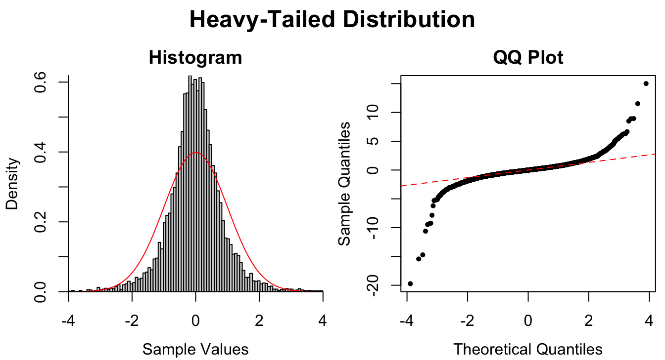
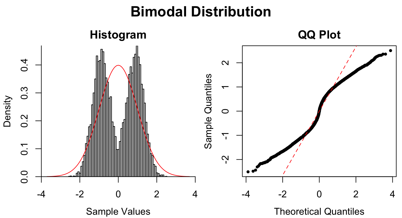
Figure 1.9: Common patterns of non-normality displayed in both histograms and QQ plots. Two iid normal samples with \(N = 100\) and \(N = 1000\) are included to show how sample size affects the plots.

Example 1.8 The four basic diagnostic plots for Dr. Gladstone’s data are displayed in Figure 1.10.

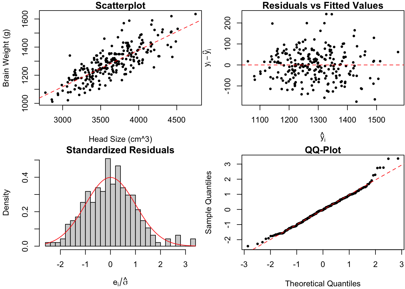
Figure 1.10: Diagnostic plots for Dr.~Gladstone’s brain data.

There is perhaps a slight increase of the spread in residuals as the fitted values increases, mildly suggesting that the variance is not constant. Furthermore, the standardized residuals are slightly right-skewed. However, it’s difficult to say whether this is simply due to random chance (see for instance the top left panel of Figure 1.9). Overall, I’m inclined to say that Dr. Gladstone’s \(n = 236\) observations fail to provide strong evidence against the linear regression assumptions -.

#--- code for Figure 10 ---------------------------------------------------

# reassign y and x to brain data
x <- brain$head.size # head size
y <- brain$brain.wgt # brain weight
M <- lm(y ~ x) # fit linear model

par(mfrow = c(2,2), mar = c(4,4,1,0)+.1)
cex <- .7
pch <- 16
# scatterplot
plot(x, y, cex = cex, pch = pch,
     xlab = "Head Size (cm^3)", ylab = "Brain Weight (g)",
     main = "Scatterplot")
abline(M, col = "red", lty = 2) # add regression line
# residuals vs fitted values
  plot(predict(M), residuals(M), cex = cex, pch = pch,
       xlab = expression(hat(y)[i]), # how to plot math symbols
       ylab = expression(y[i] - hat(y)[i]), # ?plotmath for details
       main = "Residuals vs Fitted Values")
abline(h = 0, col = "red", lty = 2) # horizontal line
# standardized residuals
zres <- residuals(M)
sig.hat <- sqrt(sum(zres^2)/length(zres-2))
zres <- zres/sig.hat
# histogram
hist(zres, breaks = 40, freq = FALSE,
     xlab = expression(e[i]/hat(sigma)),
     main = "Standardized Residuals")
curve(dnorm, add = TRUE, col = "red") # theoretical N(0,1) distribution
# QQ-plot
qqnorm(zres, main = "QQ-Plot", cex = cex, pch = pch)
qqline(zres, col = "red", lty = 2)

1.7 Appendix: \(\R\) Code for Examples

# load the brain data
brain <- read.csv(file = "brainhead.csv")
x <- brain$head.size # head size
y <- brain$brain.wgt # brain weight

# plot just points
par(mai = c(.82, .82, .1, .1))
plot(x, y, xlab = "Head Size (cm^3)", ylab = "Brain Weight (g)",
     pch = 16, cex = .7)

# simple linear regression formula for slope b1 and intercept b0:
b1.hat <- cov(x, y)/var(x)
b0.hat <- mean(y) - b1.hat * mean(x)

# add the line of best fit and vertical distances to the actual points
abline(a = b0.hat, b = b1.hat, col = "red")
segments(x0 = x, y0 = b0.hat + b1.hat*x, y1 = y, lty = 2, col = "grey")
# replot points on top of lines so it looks nicer
points(x, y, pch = 16, cex = .7)

# prediction intervals for 20 observations

m <- 20 # subset of full data

# estimates of beta0, beta1, sigma
b1.hat <- cov(x[1:m], y[1:m])/var(x[1:m])
b0.hat <- mean(y[1:m]) - b1.hat * mean(x[1:m])
sigma.hat <- sqrt(sum((y[1:m] - b0.hat - b1.hat*x[1:m])^2)/(m-2))

# prediction intervals

conf <- .95
qa <- qt(1-(1-conf)/2, df = m-2) # t_{n-2,alpha}
S.xx <- var(x[1:m])*(m-1)
x.bar <- mean(x[1:m])

# range of interval calculation
xlim <- range(x[1:m])
xlim <- (xlim-mean(xlim)) * 3 + mean(xlim) # 3x range of data

# intervals
xr <- seq(min(xlim), max(xlim), len = 1e3) # x values at which to calculate PI's
sx <- sigma.hat * sqrt(1 + 1/m + (xr-x.bar)^2/S.xx) # scale for PI's
L <- b0.hat + b1.hat*xr - qa * sx # lower bound
U <- b0.hat + b1.hat*xr + qa * sx # upper bound

# plot
par(mai = c(.82, .82, .2, .2)) # removes some white space from margins
plot(x[1:m], y[1:m], xlab = "Head Size (cm^3)", ylab = "Brain Weight (grams)",
     pch = 16, cex = .7, xlim = xlim, ylim = range(L, U))
abline(a = b0.hat, b = b1.hat, col = "red")
lines(x = xr, y = L, col = "red", lty = 2)
lines(x = xr, y = U, col = "red", lty = 2)

References

Gladstone, Reginald J. 1905. “A Study of the Relations of the Brain to the Size of the Head.” Biometrika 4 (1/2): 105–23.

Legendre, Adrien-Marie. 1805. Nouvelles Méthodes Pour La détermination Des Orbites Des Comètes. Firmin Didot: Paris.