3 Multiple Linear Regression: Case Studies

In the following examples, we shall cover some of the basic tools and techniques of regression analysis in $\R$.

3.1 Reading a Regression Output

The dataset satisfaction.csv contains four variables collected from $n = 46$ patients in given a hospital:

Satisfaction: The degree of satisfaction with the quality of care (higher values indicated greater satisfaction).
Age: The age of the patient in years.
Severity: The severity of the patient’s condition (higher values are more severe).
Stress: The patient’s self-reported degree of stress (higher values are more stress).

Let’s start by fitting the multiple linear regression model \[\begin{equation} \mtt{Satisfaction}_i = \beta_0 + \beta_1 \cdot \mtt{Age}_i + \beta_2 \cdot \mtt{Severity}_i + \beta_3 \cdot \mtt{Stress}_i + \eps_i. \tag{3.1} \end{equation}\] Model (3.1) has three covariates (Age, Severity, Stress), but the design matrix $X$ has four columns, \[ X = \begin{bmatrix} 1 & \mtt{Age}_1 & \mtt{Severity}_1 & \mtt{Stress}_1 \\ 1 & \mtt{Age}_2 & \mtt{Severity}_2 & \mtt{Stress}_2 \\ \vdots & & & \vdots \\ 1 & \mtt{Age}_{46} & \mtt{Severity}_{46} & \mtt{Stress}_{46} \end{bmatrix}, \] such that $p = 4$. The $\R$ code for fitting this model is:

# load the data
satis <- read.csv("satisfaction.csv")

# fit the linear model
M <- lm(formula = Satisfaction ~ Age + Severity + Stress,
        data = satis)
M # display coefficients

## 
## Call:
## lm(formula = Satisfaction ~ Age + Severity + Stress, data = satis)
## 
## Coefficients:
## (Intercept)          Age     Severity       Stress  
##     158.491       -1.142       -0.442      -13.470

3.1.1 Basic Components of a Regression Output

Table 3.1 displays the output of the summary(M) command.

summary(M) # summary of regression results

##
## Call:
## 
## lm(formula = Satisfaction ~ Age + Severity + Stress, data = satis)
## 
## Residuals:
##      Min       1Q   Median       3Q      Max
## -18.3524  -6.4230   0.5196   8.3715  17.1601
## 
## Coefficients:
##             Estimate Std. Error t value Pr(>|t|)
## (Intercept) 158.4913    18.1259   8.744 5.26e-11 ***
## Age          -1.1416     0.2148  -5.315 3.81e-06 ***
## Severity     -0.4420     0.4920  -0.898   0.3741
## Stress      -13.4702     7.0997  -1.897   0.0647 .
## ---
## Signif. codes:  0 '***' 0.001 '**' 0.01 '*' 0.05 '.' 0.1 ' ' 1
## 
## Residual standard error: 10.06 on 42 degrees of freedom
## Multiple R-squared:  0.6822,    Adjusted R-squared:  0.6595
## F-statistic: 30.05 on 3 and 42 DF,  p-value: 1.542e-10

The meaning of some of the terms in this output are:

Estimate: These are the $\hat \beta = (X'X)^{-1}X'y$. To interpret each $\beta_j$, recall that for multiple linear regression we have $\E[y \mid x] = x' \beta$. Therefore, if $x$ and $\tilde x$ are two covariate values that differ only by one unit in covariate $j$, i.e., \[ \tilde x - x = (0, \ldots, 0, \underset{\substack{\uparrow\\\rlap{\text{covariate $j$}}}}{1}, 0, \ldots 0), \] then $\E[y \mid \tilde x] - \E[y \mid x] = \beta_j$. In other words, $\beta_j$ is the effect on the mean of a change of 1 unit of covariate $j$ if all other covariates are held the same. For example, $\beta_\tx{Age}$ is the change per extra year of age in expected Satisfaction for two people with the same Severity and same Stress values, regardless of what these values are.
Std. Error: These are the so-called standard errors of $\hat \beta$. The standard error $\se(\hat \beta_j)$ of $\hat \beta_j$ defined as a sample-based approximation of the estimator’s standard deviation, $\sd(\hat\beta_j) = \sqrt{\var(\hat\beta_j)}$. In the regression context, we have $\var(\hat \beta) = \sigma^2 (X'X)^{-1}$, such that $\var(\hat \beta_j)$ is the $j$ diagonal element of this variance matrix: \[ \var(\hat \beta_j) = \sigma^2 [\ixtx]_{jj}. \] Therefore, a natural choice for the standard error of $\hat \beta_j$ is \[ \se(\hat \beta_j) = \hat \sigma \sqrt{\ixtx]_{jj}}. \] That is, we simply replace the unknown $\sigma$ by the square-root of the unbiased estimator.
t value: The values of the test statistics for each null hypothesis $H_0: \beta_j = 0$. These are calculated as \[ T_j = \frac{\hat \beta_j}{\tx{se}(\hat \beta_j)}. \]
Pr(>|t|): The $p$-value for each of these null hypotheses. To obtain these, recall that under $H_0: \beta_j = 0$, \[ Z = \frac{\hat \beta_j}{\sigma \sqrt{[(X'X)^{-1}]_{jj}}} \sim \N(0, 1), \qquad W = \frac{n-p}{\sigma^2}\cdot \hat \sigma^2 \sim \chi^2_{(n-p)}, \] and since $\hat \beta_j$ and $\hat \sigma^2$ are independent, so are $Z$ and $W$. Therefore, \[ \frac{Z}{\sqrt{W/(n-p)}} = \frac{\hat \beta_j}{\hat \sigma \sqrt{[(X'X)^{-1}]_{jj}}} = \frac{\hat \beta_j}{\tx{se}(\hat \beta_j)} \sim t_{(n-p)}. \] Thus, $\R$ uses the CDF of the $t$-distribution to calculate the $p$-value \[ p_j = \Pr(\abs{T_j} > \abs{T_{j,\obs}} \mid \beta_j = 0). \]
Residual standard error: The square root of the unbiased estimator, \[ \hat \sigma = \sqrt{\frac{\sum_{i=1}^n (y_i - x_i'\hat\beta)^2}{n-p}} = \sqrt{\frac{e'e}{n-p}}. \]
degrees of freedom: The degrees of freedom for the problem, which is defined as $n-p$. Note that for this example we have 3 covariates, but $p = 4$ since we are fitting four $\beta$’s, including the intercept.

So what are the significant factors in predicting patient satisfaction with the quality of hosptical care? At first glance, the $p$-values in Table 3.1 indicate that only the patient’s age (and the intercept) are significant at the 5% level. However, these $p$-values only check whether covariates are statistically significant (i.e., there’s evidence that $\beta_j \neq 0$) in the presence of all the others. Indeed, rerunning the analysis without Severity produces:

# fit model with Severity removed
summary(lm(Satisfaction ~ Age + Stress, data = satis))

## 
## Call:
## lm(formula = Satisfaction ~ Age + Stress, data = satis)
## 
## Residuals:
##      Min       1Q   Median       3Q      Max 
## -19.4453  -7.3285   0.6733   8.5126  18.0534 
## 
## Coefficients:
##             Estimate Std. Error t value Pr(>|t|)    
## (Intercept) 145.9412    11.5251  12.663 4.21e-16 ***
## Age          -1.2005     0.2041  -5.882 5.43e-07 ***
## Stress      -16.7421     6.0808  -2.753  0.00861 ** 
## ---
## Signif. codes:  0 '***' 0.001 '**' 0.01 '*' 0.05 '.' 0.1 ' ' 1
## 
## Residual standard error: 10.04 on 43 degrees of freedom
## Multiple R-squared:  0.6761, Adjusted R-squared:  0.661 
## F-statistic: 44.88 on 2 and 43 DF,  p-value: 2.98e-11

In other words, Stress is not statistically significant in the presence of both Age and Severity, but if Severity is removed, then Stress adds statistically significant predictive power to the linear model containing only Age and the intercept.

3.1.2 Coefficient of Determination

Researchers are often interested in understanding how well a model explains the observed data. To this end, recall that for response $y$, model matrix $X$, and residual vector $e$, we showed that \[ e'e = y'y - \hat \beta' X'X \hat \beta \implies y'y = \hat \beta' X'X \hat \beta + e'e. \] By subtracting $n \bar y^2$ from each side of this equality we obtain the following decomposition: \[\begin{align} y'y - n \bar y^2 & = (\hat \beta' X'X \hat \beta - n \bar y^2) + e'e, \nonumber \\ \sumi 1 n (y_i - \bar y)^2 & = \left(\sumi 1 n (x_i'\hat\beta)^2 - n \bar y^2\right) + \sumi 1 n (y_i - x_i'\hat\beta)^2. \tag{3.2} \end{align}\]

The Sum of Squares decomposition (3.2) takes on a special meaning when an intercept term $\beta_0$ is included in the model.

Proposition 3.1 Suppose the linear model $y \sim \N(X\beta, \sigma^2)$ contains an intercept term. That is, the first column of $X$ consists of all ones. Then \[ \sumi 1 n (x_i'\hat\beta)^2 - n \bar y^2 = \sumi 1 n(x_i'\hat\beta - \bar y)^2. \]

Proof. Recall that for any constant vector $a = (\rv a p)$, we have \[ (Xa)' X\hat \beta = a'X'X\ixtx X'y = a'X'y = (Xa)'y. \] Since the first column of $X$ is all ones, with $a = (\tfrac 1 n, 0, \ldots 0)$ we have $Xa = (\tfrac 1 n, \ldots \tfrac 1 n)$, such that \[ (Xa)' X\hat \beta = \frac 1 n \sumi 1 n (x_i' \hat \beta) = (Xa)' y = \frac 1 n \sumi 1 n y_i = \bar y. \] Therefore, \[\begin{align*} \textstyle \sumi 1 n (x_i'\hat \beta - \bar y)^2 & = \textstyle \sumi 1 n \left[x_i'\hat\beta - \frac 1 n \sum_{j=1}^n x_j'\hat\beta \right]^2 \\ & = \textstyle \sumi 1 n (x_i'\hat\beta)^2 - n \left(\frac 1 n \sum_{j=1}^n x_j'\hat\beta\right)^2 = \sumi 1 n (x_i'\hat\beta)^2 - n \bar y^2. \end{align*}\]

The terms in (3.2) are named as follows:

The term $\sst = \sumi 1 n (y_i - \bar y)^2$ is the Total Sum of Squares.
The term $\sse = \sumi 1 n (y_i - x_i'\hat\beta)^2$, in some sense, corresponds to the model prediction error. That is, how far are the actual values $y_i$ from their predicted values $\hat y_i = x_i'\hat \beta$. For this reason, this term is called the Error Sum of Squares or “residual sum of squares”.
The term $\ssr = \sumi 1 n (x_i'\hat \beta - \bar y)^2$ is called the Regression Sum of Squares.

In fact, $\ssr$ can be thought of as the “explained sum of squares” in light of the following argument.

Given the regression model \[\begin{equation} y_i \mid x_i \ind \N(x_i'\beta, \sigma^2), \tag{3.3} \end{equation}\] we have so far considered the $x_i$ to be fixed. However, in most applications we would not be able to control the values of the covariates. For instance, in the hospital satisfaction example, the 46 patients (presumably) were randomly sampled, leading to random values of Age, Severity, and Stress. If we consider the $x_i \iid f_X(x)$ to be randomly sampled from some distribution $f_X(x)$, then the $y_i \iid f_Y(y)$ are also being randomly sampled from a distribution \[ f_Y(y) = \int f_{Y\mid X}(y\mid x) f_X(x) \ud x, \] where the conditional distribution $f_{Y\mid X}(y\mid x)$ is the PDF of the normal distribution $y \mid x \sim \N(x'\beta, \sigma^2)$ implied by the regression model (3.3). In this sense the variance $\sigma^2_y = \var(y)$ can be defined without conditioning on $x$. In fact, the mean and variance in (3.3) are in fact the conditional mean and variance of $y$: \[ x_i'\beta = \E[y_i \mid x_i] \and \sigma^2 = \var(y_i \mid x_i). \] Let us now recall the law of double variance: \[ \var(y) = \E[\var(y \mid x)] + \var(\E[y \mid x]). \] If $y$ is “well predicted” by $x$, then $\E[y \mid x]$ is close to $y$ and $\var(\E[y \mid x])/\var(y) \approx 1$. If $y$ is “not well predicted” by $x$, then $\E[y \mid x]$ shouldn’t change too much with $x$, such that $\var(\E[y \mid x])/\var(y) \approx 0$. Based on these considerations, a measure of the quality of a linear model is \[\begin{equation} \frac{\var(\E[y \mid x])}{\var(y)} = 1 - \frac{\E[\var(y \mid x)]}{\var(y)} = 1 - \frac{\sigma^2}{\sigma^2_y}. \tag{3.4} \end{equation}\] This is commonly referred to as the “fraction of variance explained by the model”. A sample-ased measure of this quantity is the so-called coefficient of determination: \[\begin{equation} R^2 = 1 - \frac{\sse}{\sst}. \tag{3.5} \end{equation}\] This value is reported as the Multiple R-squared in Table 3.1. When the intercept is included in the model, we’ve seen that $\frac 1 n \sumi 1 n x_i'\hat\beta = \bar y$, such that if $e_i = y_i - x_i'\hat \beta$ denotes the $i$th residual, then \[ \bar e = \frac 1 n \sumi 1 n (y_i - x_i'\hat \beta) = \bar y - \bar y = 0 \implies \sumi 1 n (y_i - x_i'\hat\beta)^2 = \sumi 1 n (e_i - \bar e)^2, \] such that \[ R^2 = 1 - \frac{\sse/(n-1)}{\sst/(n-1)} = 1 - \frac{\frac 1 {n-1} \sumi 1 n (y_i - x_i'\hat \beta)^2}{\frac 1 {n-1} \sumi 1 n (y_i - \bar y)^2} \] can be written in terms of the sample variances of $e$ and $y$. If, however, the goal is to estimate $1 - \sigma^2/\sigma^2_y$, then the numerator should employ the unbiased estimator $\hat \sigma^2$. This leads to the adjusted coefficient of determination \[ R^2_\tx{adj} = 1 - \frac{\hat \sigma^2}{\sst/(n-1)}. \] This value is reported as Adjusted R-squared in Table 3.1.

3.2 Basic Nonlinear Models

The dataset tortoise.csv contains 18 measurements of tortoise hatch yields as a function of size. Specifically, the dataset contains the variables:

NumEggs: the number of eggs in the tortoise’s hatch
CarapDiam: the diameter of its carapace (cm)

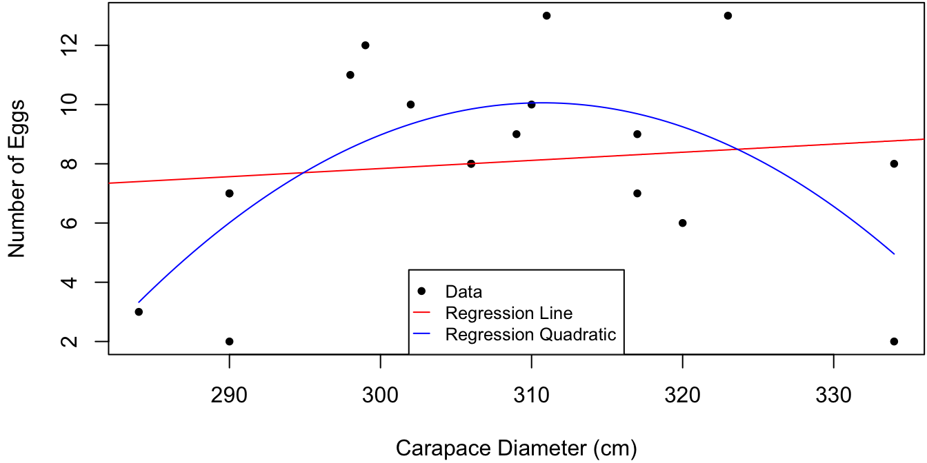
Figure 3.1: Hatch size as a function of tortoise carapace size. Linear and quadratic regression fits are plotted in red and blue, respectively.

The data in Figure 3.1 is poorly described by a straight regression line and has only marginal significance.

tortoise <- read.csv("tortoise.csv") # load data
# fit a linear model in CarapDiam
M1 <- lm(NumEggs ~ CarapDiam, data = tortoise)
summary(M1)

## 
## Call:
## lm(formula = NumEggs ~ CarapDiam, data = tortoise)
## 
## Residuals:
##     Min      1Q  Median      3Q     Max 
## -6.7790 -1.1772 -0.0065  2.0487  4.8556 
## 
## Coefficients:
##             Estimate Std. Error t value Pr(>|t|)
## (Intercept) -0.43532   17.34992  -0.025    0.980
## CarapDiam    0.02759    0.05631   0.490    0.631
## 
## Residual standard error: 3.411 on 16 degrees of freedom
## Multiple R-squared:  0.01478,    Adjusted R-squared:  -0.0468 
## F-statistic:  0.24 on 1 and 16 DF,  p-value: 0.6308

A second look at Figure 3.1 reveals that hatch size increases and then decreases as a function of carapace size. It turns out that shell of a tortoise increases throughout its lifetime, whereas its fertility increases up to a certain point and then starts decreasing. This nonlinear trend can be captured using the linear modeling machinery by adding a quadratic term to the regression. That is, we can fit a model of the form \[ \mtt{NumEggs}_i = \beta_0 + \beta_1 \mtt{CarapDiam}_i + \beta_2 \mtt{CarapDiam}_i^2 + \eps_i, \quad \eps_i \iid \N(0, \sigma^2). \] The $\R$ command for fitting this model is

M2 <- lm(NumEggs ~ CarapDiam + I(CarapDiam^2), data = tortoise)
summary(M2)

## 
## Call:
## lm(formula = NumEggs ~ CarapDiam + I(CarapDiam^2), data = tortoise)
## 
## Residuals:
##     Min      1Q  Median      3Q     Max 
## -4.0091 -1.8480 -0.1896  2.0989  4.3605 
## 
## Coefficients:
##                  Estimate Std. Error t value Pr(>|t|)   
## (Intercept)    -8.999e+02  2.703e+02  -3.329  0.00457 **
## CarapDiam       5.857e+00  1.750e+00   3.347  0.00441 **
## I(CarapDiam^2) -9.425e-03  2.829e-03  -3.332  0.00455 **
## ---
## Signif. codes:  0 '***' 0.001 '**' 0.01 '*' 0.05 '.' 0.1 ' ' 1
## 
## Residual standard error: 2.671 on 15 degrees of freedom
## Multiple R-squared:  0.4338, Adjusted R-squared:  0.3583 
## F-statistic: 5.747 on 2 and 15 DF,  p-value: 0.01403

Note the use of the “as is” function I(). This is because operations such as "+,-,*,:" have a different meaning in formula objects, which is the first argument to lm:

args(lm)

## function (formula, data, subset, weights, na.action, method = "qr", 
##     model = TRUE, x = FALSE, y = FALSE, qr = TRUE, singular.ok = TRUE, 
##     contrasts = NULL, offset, ...) 
## NULL

This simple example serves to illustrate the great flexibility of linear models. Indeed, we can use regression methods to fit any model of the form \[ y_i = \sum_{j=1}^p \beta_j f_j(x_i) + \eps_i, \quad \eps_i \iid \N(0, \sigma^2), \] where the $f_j(x)$ are predetermined functions which can be arbitrarily nonlinear. However, I would not recommend to e.g., include terms of the form $x, x^2, x^3, \ldots$ to capture an unknown nonlinear effect in the response. Typically $x$ and $x^2$ are sufficient and if not there is most likely something else going on that requires further (graphical) investigation.

$\R$ code to produce Figure 3.1:

par(mar = c(4, 4, 0, 0) + .1) # reduce plot margin size
plot(tortoise$CarapDiam, tortoise$NumEggs, pch = 16, cex = .8,
     xlab = "Carapace Diameter (cm)", ylab = "Number of Eggs") # raw data
abline(M1, col = "red") # line of best fit
curve(M2$coef[1] + M2$coef[2]*x + M2$coef[3]*x^2,
      col = "blue", add = TRUE) # quadratic of best fit
legend(x = "bottom", legend = c("Data", "Regression Line", "Regression Quadratic"),
       pch = c(16, NA, NA), pt.cex = .8, cex = .8, col = c("black", "red", "blue"),
       lty = c(NA, 1, 1), seg.len = 1) # legend

3.2.1 Interpretation of the Intercept

In the non-linear regression example above, we have $\E[y \mid x] = \beta_0 + \beta_1 x + \beta_2 x^2$. So how to interpret the parameters? We can use complete-the-square to write \[\begin{align*} \E[y \mid x] & = \beta_2(x + \tfrac 1 2 \beta_1/\beta2)^2 - \tfrac 1 4 \beta_1^2/\beta_2 + \beta_0, \end{align*}\] such that $\gamma = -\tfrac 1 2 \beta_1\beta_2$ is the shell size at which tortoises produce the maximum expected number of eggs, and $\beta_2$ is the quadrature of the expected value at the mode. But what about $\beta_0$? We have $\E[y \mid x = 0] = \beta_0$, such that $\beta_0$ is the expected number of eggs for a tortoise of size zero. Thus, $\beta_0$ in this model does not have a meaningful interpretation. One way to change this is to shift the $x$ values in the regression. That is, consider the regression model \[ y_i = \gamma_0 + \gamma_1 (x-a) + \gamma_2 (x-a)^2 + \eps_i, \] where $a$ is a pre-specified constant. Then the intercept of this model $\gamma_0$ is the expected number of eggs for a tortoise of size $a$. The following code show how to fit this regression where $a$ is the mean of the observed shell sizes.

M2b <- lm(NumEggs ~ I(CarapDiam-mean(CarapDiam)) + I((CarapDiam-mean(CarapDiam))^2),
          data = tortoise)
# alternately we can add a covariate to the dataframe
tortoise$CarapDiam2 <- tortoise$CarapDiam - mean(tortoise$CarapDiam)
M2b <- lm(NumEggs ~ CarapDiam2 + I(CarapDiam2^2), data = tortoise)
coef(M2b)

##     (Intercept)      CarapDiam2 I(CarapDiam2^2) 
##     9.976717561     0.055623247    -0.009424876

Thus, the estimated mean number of eggs for a tortoise of average size is 9.98. Interestingly, the shifted and unshifted quadratic regression models have exactly the same predicted values:

range(predict(M2) - predict(M2b))

## [1] -1.717737e-12 -4.369838e-13

3.3 Categorical Predictors

The dataset fishermen_mercury.csv contains data on the mercury concentration found in $n = 135$ Kuwaiti villagers. Some of the variables in the dataset are:

fisherman: Whether or not the subject is a fisherman: 1 = yes, 0 = no.
age: Age of the subject (years).
height: Height (cm).
weight: Weight (kg).
fishmlwk: Number of fish meals per week.
fishpart: Parts of fish consummed: 0 = none, 1 = muscle tissue only, 2 = muscle tissue and sometimes whole fish, 3 = whole fish.
MeHg: Concentration of methyl mercury extracted from subject’s hair sample (mg/g).

Suppose we wish to predict MeHg as a function of fishpart. The variable fishpart is called a categorical predictor (as opposed to a continuous variable) as it only takes on discrete values 0,1,2,3. Moreover, these values do not correspond to integers, but rather to non-numeric categories: none, muscle tissue only, etc. Therefore, while the $\R$ command

mercury <- read.csv("fishermen_mercury.csv")
M1 <- lm(MeHg ~ fishpart, data = mercury)

compiles without errors, it assumes that the change predicted MgHg between fishpart=0 and fishpart=1 is exactly the same as between fishpart=1 and fishpart=2:

# Estimated mean MeHg for each fishpart = 0:2
Mpred <- predict(M1, newdata = data.frame(fishpart = 0:2))
names(Mpred) <- NULL # for display purposes
# difference between fishpart = 1-0 and fishpart = 2-1
c(diff10 = Mpred[2]-Mpred[1], diff21 = Mpred[3]-Mpred[2])

##    diff10    diff21 
## 0.4614899 0.4614899

A more appropriate treatment of categorical predictors is to include a different effect for each category. This can be fit into the linear regression framework through the use of indicator variables: \[ \mtt{MeHg}_i = \beta_0 + \beta_1\cdot \tx{I}[\mtt{fishpart}_i=1] + \beta_2\cdot \tx{I}[\mtt{fishpart}_i=2] + \beta_3\cdot \tx{I}[\mtt{fishpart}_i=3] + \eps_i. \] Here, \[ \tx{I}[\mtt{fishpart}_i=j] = \begin{cases}1 & \tx{$i$th subject has $\mtt{fishpart}=j$} \\ 0& \tx{otherwise}. \end{cases} \] Note that there is no indicator for fishpart=0. When this is the case, all three other indicators are equal to zero, such that \[ \E[\tx{MeHg} \mid \mtt{fishpart} = j] = \begin{cases} \beta_0, & j = 0 \\ \beta_0 + \beta_j, & j > 0. \end{cases} \] The corresponding regression model is fit in $\R$ by first converting fishpart to a factor object:

fishpart <- mercury$fishpart
head(fishpart) # original values

## [1] 2 1 2 1 1 1

fpnames <- c("none", "tissue_only", "tissue+whole", "whole") # new values

# encode the factor
fishpart2 <- rep(NA, length(fishpart)) # allocate space
for(ii in 0:3) {
  fishpart2[fishpart == ii] <- fpnames[ii+1]
}
head(fishpart2) # as a character vector

## [1] "tissue+whole" "tissue_only"  "tissue+whole" "tissue_only"  "tissue_only" 
## [6] "tissue_only"

fishpart2 <- factor(fishpart2, levels = fpnames)
head(fishpart2) # as a factor object

## [1] tissue+whole tissue_only  tissue+whole tissue_only  tissue_only 
## [6] tissue_only 
## Levels: none tissue_only tissue+whole whole

# a different way of creating the character vector is
# to index the corresponding elements of fpnames
fishpart2 <- fpnames[fishpart+1] # none = 1, tissue_only = 2, etc.
fishpart2 <- factor(fishpart2, levels = fpnames)

# fit the regression
mercury$fishpart <- fishpart2
M <- lm(MeHg ~ fishpart, data = mercury)
summary(M)

## 
## Call:
## lm(formula = MeHg ~ fishpart, data = mercury)
## 
## Residuals:
##     Min      1Q  Median      3Q     Max 
## -4.5307 -1.6041 -0.4657  0.8548 12.2963 
## 
## Coefficients:
##                      Estimate Std. Error t value Pr(>|t|)    
## (Intercept)            0.9040     0.8529   1.060  0.29115    
## fishparttissue_only    4.0137     0.9936   4.039 9.08e-05 ***
## fishparttissue+whole   2.5187     0.9001   2.798  0.00591 ** 
## fishpartwhole          3.9846     1.2393   3.215  0.00164 ** 
## ---
## Signif. codes:  0 '***' 0.001 '**' 0.01 '*' 0.05 '.' 0.1 ' ' 1
## 
## Residual standard error: 2.697 on 131 degrees of freedom
## Multiple R-squared:  0.1271, Adjusted R-squared:  0.1071 
## F-statistic: 6.357 on 3 and 131 DF,  p-value: 0.0004673

The design matrix $X$ for this regression can be obtained through the command

tail(model.matrix(M)) # tail: bottom 6 rows

##     (Intercept) fishparttissue_only fishparttissue+whole fishpartwhole
## 130           1                   0                    0             0
## 131           1                   0                    1             0
## 132           1                   0                    1             0
## 133           1                   0                    1             0
## 134           1                   1                    0             0
## 135           1                   0                    0             0

This reveals that observation 131 has fishpart = tissue+whole, whereas observations 130 and 135 have fishpart = none. Alternatively, we can fit the model with individual coefficients for each level of fishpart by forcibly removing the intercept from the model:

# "minus" removes covariates, in this case, the intercept.
M2 <- lm(MeHg ~ fishpart - 1, data = mercury)
coef(M2)

##         fishpartnone  fishparttissue_only fishparttissue+whole 
##             0.904000             4.917714             3.422739 
##        fishpartwhole 
##             4.888556

3.3.1 Significance of Multiple Predictors

Consider the linear model \[ \mtt{MeHg}_i = \mtt{fishmlwk}_i + \mtt{fishpart}_i + \eps_i, \quad \eps_i \iid \N(0, \sigma^2). \] We have seen that the $p$-value of fishmlwk contained in the Pr(>|t|) column of the regression summary indicates the statistical significance of fishmlwk as a predictor when fishpart is included in the model. That is, Pr(>|t|) measures the probability of obtaining more evidence against $H_0: \beta_{\mtt{fishmlwk}} = 0$ than we found in the present dataset.

Question: How to now test the reverse, i.e., whether fishpart significantly improves predictions when fishmlwk is part of the model?

To answer this, let’s consider a more general problem. Suppose we have the linear regression model \[ y \sim \N(X \beta, \sigma^2 I) \quad \iff \quad y_i \mid x_i \ind \N\big(\textstyle\sum_{j=1}^p x_{ij} \beta_j, \sigma^2\big), \quad i = 1,\ldots, n. \] Now we wish to test whether $q < p$ of the coefficients, let’s say $\rv \beta q$, are all equal to zero: \[ H_0: \beta_j = 0, \ 1 \le j \le q. \]

Setting up the null hypothesis is the first step. The next step is to measure evidence against $H_0$. We could use $\max_{1\le j\le q} |\hat \beta_j|$, or perhaps $\sum_{j=1}^q \hat\beta_j^2$. In some sense, the second measure of evidence is more sensitive than the first, but why weight the $\hat \beta_j^2$ equally since they have different standard deviations? Indeed, recall that $\hat \beta \sim \N(\beta, \sigma^2 (X'X)^{-1})$. Now, let $\gamma = (\rv \beta q)$ and $\hat \gamma = (\rv {\hat \beta} q)$. Then \[ \hat \gamma \sim \N(\gamma, \sigma^2 V), \] where $V_{q\times q}$ are the top-left entries of $(X'X)^{-1}$. Recall that $Z = L^{-1}(\hat \gamma - \gamma) \sim \N(0, I_q)$, where $\sigma^2 V = LL'$. Thus, if $Z = (\rv Z q)$, we have \[ \sum_{j=1}^q Z_j^2 = Z'Z = (\hat \gamma - \gamma)'(L^{-1})'L^{-1}(\hat \gamma - \gamma) = \frac 1 {\sigma^2} (\hat \gamma - \gamma)'V^{-1}(\hat \gamma - \gamma). \] So under $H_0: \gamma = 0$, we have \[ x_1 = \frac 1 {\sigma^2} \hat \gamma'V^{-1}\hat \gamma = \sum_{j=1}^q Z_j^2 \sim \chi^2_{q}. \] Moreover, this is independent of \[ x_2 = \frac {n-p} {\sigma^2} \hat \sigma^2 \sim \chi^2_{(n-p)}. \] The commonly used measure of evidence against $H_0: \gamma = 0$ is given by \[\begin{equation} F = \frac{x_1/q}{x_2/(n-p)} = \frac{\hat \gamma' V^{-1} \hat \gamma}{q\hat \sigma^2}. \tag{3.6} \end{equation}\] Thus, $F$ is a (scaled) ratio of independent chi-squared random variables and its distribution does not depend on the values of $\alpha = (\rv [q+1] \beta p)$ when $H_0$ is true. The distribution of $F$ under $H_0$ is so important that it gets its own name.

Definition 3.1 Suppose that $X_1 \sim \chi^2_{(\nu_1)}$ and independently $X_2 \sim \chi^2_{(\nu_2)}$. Then the ratio \[ W = \frac{X_1/\nu_1}{X_2/\nu_2} \] is said to have an $F$-distribution and this is denoted $W \sim \mathcal F(\nu_1, \nu_2)$. The PDF of $W$ is given by \[ f_W(w) = \frac{\Gamma(\tfrac {\nu_1+\nu_2} 2)}{\Gamma(\tfrac {\nu_1}2)\Gamma(\tfrac {\nu_2}2)} \sqrt{\nu_1^{\nu_1} \nu_2^{\nu_2} \frac{w^{\nu_1-2}}{(\nu_2 + \nu_1 w)^{(\nu_1+\nu_2)}}}. \]

3.3.2 Full and Reduced Models

The so-called “$F$-statistic” defined in (3.6) can be derived from a different perspective. That is, suppose that we partition the design matrix $X$ as \[ X_{n\times p} = [W_{n\times q} \mid Z_{n\times(p-q)}]. \] Then for $\gamma = (\rv \beta q)$ and $\alpha = (\rv [q+1] \beta p)$, the regression model can be written as \[ M_\tx{full}: y \sim \N(X\beta, \sigma^2 I) \iff y \sim \N(W \gamma + Z \alpha, \sigma^2 I). \] Under the null hypothesis $H_0: \gamma = 0$, we are considering the “reduced” model \[ M_\tx{red}: y \sim \N(Z\alpha, \sigma^2 I). \] Notice that $M_\tx{red}$ is nested in $M_\tx{full}$. That is, $M_\tx{red}$ is within the family of models specified by $M_\tx{full}$, under the restriction that the first $q$ elements of $\beta$ are equal to zero. It turns out that if ${\sse}\sp{\tx{full}}$ and ${\sse}\sp{\tx{red}}$ are the residual sum-of-squares from the full and reduced models, then the numerator of the $F$-statistic in (3.6) can be written as \[ \hat \gamma' V^{-1} \hat \gamma = {\sse}\sp{\tx{red}} - {\sse}\sp{\tx{full}}. \] If we let $\tx{df}_\tx{full} = n - p$ and $\tx{df}_\tx{red} = n - (p-q)$ denote the degrees of freedom in each model, then we may write \[\begin{equation} F = \frac{({\sse}\sp{\tx{red}} - {\sse} \sp{\tx{full}})/(\tx{df}_\tx{red}-\tx{df}_\tx{full})}{ {\sse}\sp{\tx{full}}/\tx{df}_{\tx{full}}}. \tag{3.7} \end{equation}\] Indeed, this is the method that $\R$ uses to to calculate the $F$-statistic:

Mfull <- lm(MeHg ~ fishmlwk + fishpart, data = mercury) # full model
Mred <- lm(MeHg ~ fishmlwk, data = mercury) # reduced model

# calculate F-statistic by hand
coef(Mfull) # the last 3 coefficients are those corresponding to fishpart

##          (Intercept)             fishmlwk  fishparttissue_only 
##            0.9040000            0.1073004            3.1399827 
## fishparttissue+whole        fishpartwhole 
##            1.8054351            3.1738417

null.ind <- 3:5 # which coefficients are set to 0 under H0
gam.hat <- coef(Mfull)[null.ind]
V <- solve(crossprod(model.matrix(Mfull))) # (X'X)^{-1}
V <- V[null.ind,null.ind] # var(gam.hat)/sigma^2
sigma2.hat <- sum(resid(Mfull)^2)/Mfull$df
q <- length(null.ind)
Fobs <- crossprod(gam.hat, solve(V, gam.hat))/(q*sigma2.hat)
pval <- pf(Fobs, df1 = q, df2 = Mfull$df, lower.tail = FALSE) # p(Fobs > F | H0)
c(Fstat = Fobs, pval = pval) # display

##     Fstat      pval 
## 3.8942817 0.0105453

# using the built-in R function
anova(Mred, Mfull)

## Analysis of Variance Table
## 
## Model 1: MeHg ~ fishmlwk
## Model 2: MeHg ~ fishmlwk + fishpart
##   Res.Df    RSS Df Sum of Sq      F  Pr(>F)  
## 1    133 997.64                              
## 2    130 915.38  3    82.263 3.8943 0.01055 *
## ---
## Signif. codes:  0 '***' 0.001 '**' 0.01 '*' 0.05 '.' 0.1 ' ' 1

In the special case where the model has $p$ predictors and an intercept term, \[ y_i \mid x_i \ind \N(\beta_0 + x_i'\beta, \sigma^2), \] the $F$-statistic against the null hypothesis \[ H_0: \beta_1 = \cdots = \beta_p = 0 \] of all coefficients being equal to zero except for the intercept is \[ F = \frac{(\sst-\sse)/p}{\sse/(n-p-1)}. \] This quantity and its $p$-value are reported in Table 3.1 as F-statistic and p-value.

3.4 Interaction Effects

The dataset real_estate.txt contains the sale price of 521 houses in California and some other characteristics of the house:

SalePrice: Sale price ($).
SqrFeet: Floor area (square feet).
Bedrooms: Number of bedrooms.
Bathrooms: Number of bathrooms.
Air: Air conditioning: 1 = yes, 0 = no.
CarGarage: Size of garage (number of cars).
Pool: Is there a pool: 1 = yes, 0 = no.
Lotsize: Size of property (square feet).

The model \[ M_1: \mtt{SalePrice}_i = \beta_0 + \beta_1 \mtt{SqrFeet}_i + \beta_2 \cdot \tx{I}[\mtt{Air}_i = 1] + \eps_i, \quad \eps_i \iid \N(0,\sigma^2) \] can be fit in $\R$ with the command:

real <- read.csv("real_estate.txt")
M1 <- lm(SalePrice ~ SqrFeet + Air, data = real) # model with main effects
summary(M1)

## 
## Call:
## lm(formula = SalePrice ~ SqrFeet + Air, data = real)
## 
## Residuals:
##     Min      1Q  Median      3Q     Max 
## -233330  -39803   -7338   25765  390175 
## 
## Coefficients:
##               Estimate Std. Error t value Pr(>|t|)    
## (Intercept) -95886.952  12341.639  -7.769 4.26e-14 ***
## SqrFeet        155.323      4.974  31.226  < 2e-16 ***
## Air          26630.747   9440.052   2.821  0.00497 ** 
## ---
## Signif. codes:  0 '***' 0.001 '**' 0.01 '*' 0.05 '.' 0.1 ' ' 1
## 
## Residual standard error: 77770 on 518 degrees of freedom
## Multiple R-squared:  0.6818, Adjusted R-squared:  0.6806 
## F-statistic:   555 on 2 and 518 DF,  p-value: < 2.2e-16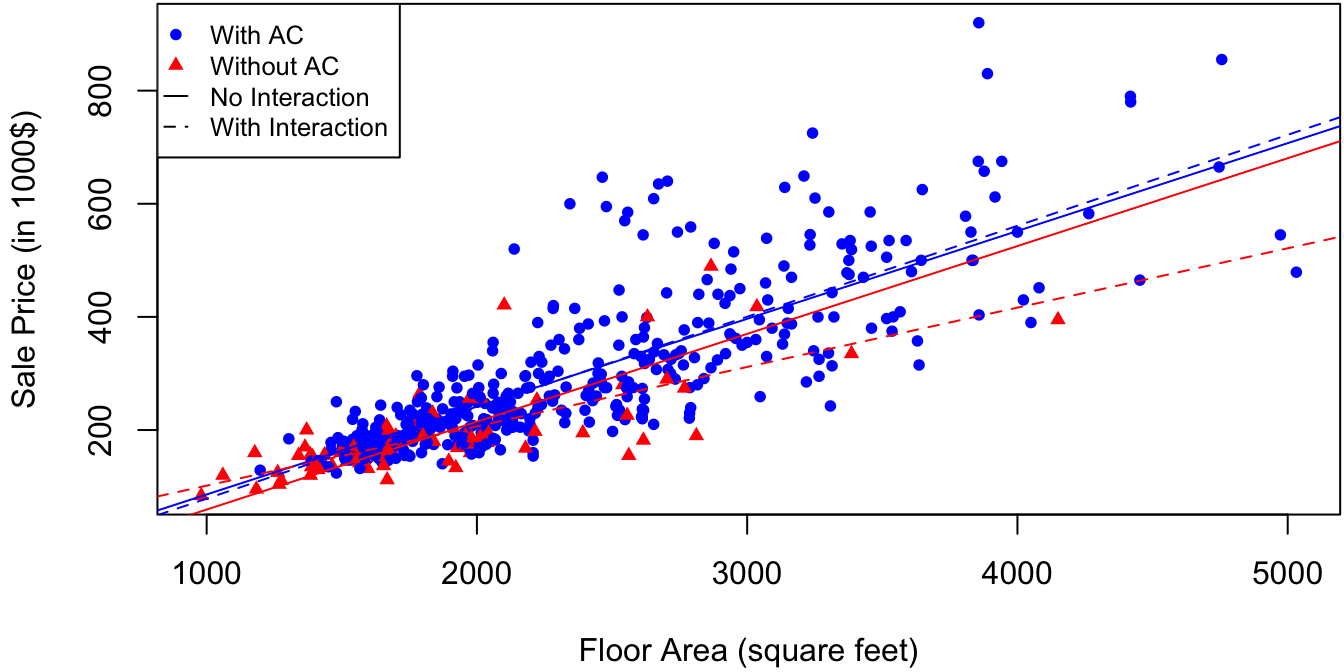

The estimated predictions for this model are the solid lines superimposed on the data in Figure 3.2.

Sale price as a function of floor area for 521 houses in California. Solid lines correspond to predictions with AC as an additive effect, and dotted lines account for interaction between AC and floor area.

Figure 3.2: Sale price as a function of floor area for 521 houses in California. Solid lines correspond to predictions with AC as an additive effect, and dotted lines account for interaction between AC and floor area.

Model $M_1$ produces parallel regression lines. That is, the increase in the expected sale price for a given house per square foot of floor area is the same for houses with and without air conditioning: \[\begin{equation} \begin{split} & \E[\mtt{SalePrice} \mid \mtt{SqrFeet} = a_2, \mtt{Air} = \color{blue}{\tx{yes}}] - \E[\mtt{SalePrice} \mid \mtt{SqrFeet} = a_1, \mtt{Air} = \color{blue}{\tx{yes}}] \\ = & \E[\mtt{SalePrice} \mid \mtt{SqrFeet} = a_2, \mtt{Air} = \color{red}{\tx{no}}] - \E[\mtt{SalePrice} \mid \mtt{SqrFeet} = a_1, \mtt{Air} = \color{red}{\tx{no}}] \\ = & \beta_1(a_2-a_1). \end{split} \tag{3.8} \end{equation}\] If we wish to model the increase in SalePrice per unit of SqrFeet differently houses with and without air-conditioning, we can do this in $\R$ with the command

M2 <- lm(SalePrice ~ SqrFeet*Air, data = real) # model with interaction effect
summary(M2)

## 
## Call:
## lm(formula = SalePrice ~ SqrFeet * Air, data = real)
## 
## Residuals:
##     Min      1Q  Median      3Q     Max 
## -248009  -37126   -7803   22249  381919 
## 
## Coefficients:
##              Estimate Std. Error t value Pr(>|t|)    
## (Intercept)  -3217.55   30085.04  -0.107 0.914871    
## SqrFeet        104.90      15.75   6.661 6.96e-11 ***
## Air         -78867.83   32663.33  -2.415 0.016100 *  
## SqrFeet:Air     55.89      16.58   3.371 0.000805 ***
## ---
## Signif. codes:  0 '***' 0.001 '**' 0.01 '*' 0.05 '.' 0.1 ' ' 1
## 
## Residual standard error: 77010 on 517 degrees of freedom
## Multiple R-squared:  0.6887, Adjusted R-squared:  0.6869 
## F-statistic: 381.2 on 3 and 517 DF,  p-value: < 2.2e-16

The formula term SqrFeet*Air expands to SqrFeet + Air + SqrFeet:Air, and this corresponds to the model \[ M_2: \mtt{SalePrice}_i = \beta_0 + \beta_1 \mtt{SqrFeet}_i + \beta_2 \cdot \tx{I}[\mtt{Air}_i = 1] + \beta_3 \big(\mtt{SqrFeet}_i\cdot \tx{I}[\mtt{Air}_i = 1]\big) + \eps_i. \] The last term in this model enters the design matrix $X$ as \[ \mtt{SqrFeet}_i\cdot I[\mtt{Air}_i = 1] = \begin{cases} 0 & \tx{house $i$ has no AC}, \\ \mtt{SqrFeet}_i & \tx{house $i$ has AC}. \end{cases} \] The predictions of model $M_2$ are the dotted lines in Figure 3.2. The output of summary(M2) indicates that SqrFeet:Air significantly increases the fit to the data in the presence of only SqrFeet and Air. The term SqrFeet:Air is called an interaction term. In its absence, SqrFeet and Air are said to enter additively into model $M_1$ in reference to equation (3.8). That is, Air has a purely additive effect in model $M_1$, since it “adds on” the same value of $\beta_2$ to the predicted sale price for any floor area. In general, we have the following:

Definition 3.2 Consider a general regression model of the form \[ y \mid x \ind \N(\mu(x), \sigma^2), \qquad x = (\rv x p). \] Covariate $x_j$ is said to have an additive effect if \[ \mu(x) = g(x_j) + h(\rv x {j-1}, \rv [j+1] x p). \] That is, if $x$ and $\tilde x$ are two covariate vectors that differ only in covariate $j$, then \[ \E[y \mid \tilde x] - \E[y \mid x] = g(\tilde x_j) - g(x_j), \] regardless of the values in the other covariates. Covariate $x_j$ is said to have an interaction effect if it does not have an additive effect. For example, if \[ \mu(x) = g(x_1, x_2) + h(\rv [3] x p), \] then we would say that there is an interaction effect between $x_1$ and $x_2$.

We can also have interactions between continuous covariates. For example, suppose that we have:

$y$: The yield of a crop.
$x$: The amount of fertilizer.
$w$: The amount of pesticide.

Then a basic interaction model is of the form \[ M: y_i = \beta_0 + \beta_1 x_i + \beta_2 w_i + \beta_3 x_i w_i + \eps_i. \] Thus for every fixed amount of fertilizer, there is a different linear relation between amount of pesticide and yield: \[ \E[y \mid x, w] = \beta_{0x} + \beta_{1x} w, \] where $\beta_{0x} = \beta_0 + \beta_1 x$ and $\beta_{1x} = \beta_2 + \beta_3 x$. This also provides an interpretation of $\beta_3$. If $\tilde x = x + 1$, then \[ \beta_3 = \beta_{1\tilde x} - \beta_{1x}. \] In other words, $\beta_3$ is the difference in the effect per unit of pesticide on yield for a change of one unit of fertilizer.

$\R$ code to produce Figure 3.2:

clrs <- c("blue", "red")
mrkr <- c(16,17)
ltype <- c(1,2)
par(mar = c(4, 4, 0, 0) + .1) # reduce plot margin size
plot(y = real$SalePrice/1000, x = real$SqrFeet, cex = .8, # size of points
     pch = mrkr[2-real$Air], col = clrs[2-real$Air], # different colors for AC/no AC
     xlab = "Floor Area (square feet)", ylab = "Sale Price (in 1000$)") # raw data
# add predictions for main effects model (M1)
beta1 <- coef(M1)/1000 # since SalePrice is in 1000$
abline(a = beta1["(Intercept)"],
       b = beta1["SqrFeet"], col = clrs[2], lty = ltype[1]) # no AC
abline(a = beta1["(Intercept)"] + beta1["Air"],
       b = beta1["SqrFeet"], col = clrs[1], lty = ltype[1]) # with AC
# add predictions for interaction effects model (M2)
beta2 <- coef(M2)/1000
abline(a = beta2["(Intercept)"],
       b = beta2["SqrFeet"], lty = ltype[2], col = clrs[2]) # no AC
abline(a = beta2["(Intercept)"] + beta2["Air"],
       b = beta2["SqrFeet"] + beta2["Air:SqrFeet"],
       lty = ltype[2], col = clrs[1]) # with AC
# add legend to plot
legend(x = "topleft",
       legend = c("With AC", "Without AC", "No Interaction", "With Interaction"),
       col = c(clrs, "black", "black"), pch = c(mrkr, NA, NA),
       cex = .8, pt.cex = .8,
       lty = c(NA, NA, ltype), seg.len = 1)

3.5 Heteroskedastic Errors

The basic regression model \[ y_i = x_i'\beta + \eps_i, \quad \eps_i \iid \N(0, \sigma^2) \] is said to have homoskedastic errors. That is, the variance of each error term $\eps_i$ is constant: $\var(\eps_i) \equiv \sigma^2$. A model with heteroskedastic errors is of the form \[ y_i = x_i'\beta + \eps_i, \quad \eps_i \ind \N(0, \sigma_i^2), \] where the error of each subject/experiment $i = 1,\ldots,n$ is allowed to have a different variance. Two common examples of heteroskedastic errors are presented below.

3.5.1 Replicated Measurements

The hospitals.csv dataset consists of measurements of post-surgery complications in 31 hospitals in New York state. The variables in the dataset are:

SurgQual: A quality index for post-surgery complications aggregated over all patients in the hospital (higher means less complications).
Difficulty: A measure of the average difficulty of surgeries for that hospital (higher means more difficult cases).
N: The number of patients used to calculate these indices.

The simple regression estimate of SurgQual as a function of Difficulty is superimposed onto the actual data in Figure 3.3. The size of each datapoint in Figure 3.3 is proportional to the number of patients used to calculate each aggregated quality score. It is natural to expect that the hospitals with many patients have their scores more accurately estimated than those with few patients. Therefore, it would seem fair to give the larger hospitals more “weight” when fitting a regression model.

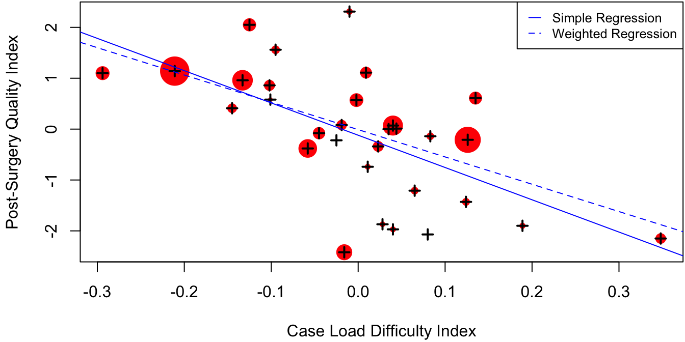
Aggregated measure of post-surgery complications as a function of difficulty of case load for 31 hospitals in New York state. The size of each data point is proportional to the number of patients used to compute the aggregate. Simple and weighted regression lines are indicated by the solid and dotted lines.

Figure 3.3: Aggregated measure of post-surgery complications as a function of difficulty of case load for 31 hospitals in New York state. The size of each data point is proportional to the number of patients used to compute the aggregate. Simple and weighted regression lines are indicated by the solid and dotted lines.

To formalize this, suppose that $y_{ij}$ is the quality score for patient $j$ in hospital $i$. If each $y_{ij}$ has common variance about the hospital mean \[ x_i'\beta = \beta_0 + \beta_1 \mtt{Difficulty}_i, \] we could model this using \[ y_{ij} = x_i'\beta + \eps_{ij}, \quad \eps_{ij} \iid \N(0,\sigma^2). \] Thus, each hospital score $\mtt{SurgQual}_i$ is an average of the scores of individual patients, \[ \mtt{SurgQual}_i = y_i = \frac 1 {N_i} \sum_{j=1}^{N_i} y_{ij}, \] such that \[\begin{equation} y_i = x_i' \beta + \eps_i, \quad \eps_i = \frac 1 {N_i} \sum_{j=1}^{N_i} \eps_{ij} \ind \N(0, \sigma^2/N_i). \tag{3.9} \end{equation}\]

To fit the “repeated measurements” model (3.9), let \[\begin{align*} \tilde y_i & = N_i^{1/2} y_i, & \tilde x_i & = N_i^{1/2} x_i, & \tilde \eps_i & = N_i^{1/2} \eps_i. \end{align*}\] Then model (3.9) becomes \[ \tilde y_i = \tilde x_i' \beta + \tilde \eps_i, \quad \tilde \eps_i \iid \N(0, \sigma^2). \] In other words, by rescaling the response and predictors by the square-root of the sample size, we can transform the heteroskedastic repeated measurements regression problem into a homoskedastic one. If $y$, $\tilde y$ and $X$, $\tilde X$ denote the original and transformed response vector and design matrix, then \[ \tilde y = D^{1/2} y \and \tilde X = D^{1/2} X, \where D = \left[\begin{smallmatrix} N_1 & & 0\\ & \ddots & \\ 0& & N_n \end{smallmatrix} \right]. \] The regression parameter estimates are then \[\begin{align*} \hat \beta & = (\tilde X' \tilde X)^{-1} \tilde X' \tilde y = (X'DX)^{-1} X'Dy, \\ \hat \sigma^2 & = \frac{\sumi 1 n (\tilde y_i - \tilde x_i'\hat \beta)^2}{n-p} = \frac{(y - X\hat\beta)'D(y - X\hat\beta)}{n-p}. \end{align*}\] This “weighted regression” is achieved in $\R$ with the weights argument to lm():

# calculate the weighted regression using matrices
y <- hosp$SurgQual # response
X <- cbind(1, hosp$Difficulty) # covariate matrix
N <- hosp$N # sample sizes

beta.hat <- c(solve(crossprod(X, X*N), crossprod(X, y*N))) # weighted MLE
beta.hat

## [1] -0.009991708 -5.368283909

# using the built-in R function
# R expects weights = N, not weights = sqrt(N)
lm(SurgQual ~ Difficulty, weights = N, data = hosp)

## 
## Call:
## lm(formula = SurgQual ~ Difficulty, data = hosp, weights = N)
## 
## Coefficients:
## (Intercept)   Difficulty  
##   -0.009992    -5.368284

Figure 3.3 indicates that weighting the hospitals proportionally to sample size attenuates the negative relationship between the post-surgery quality index and the case load difficulty index. This is because many of the low-performing hospitals with difficult case loads had few patients, whereas some of the well-performing hospitals with less difficult cases had a very large number of patients.

$\R$ code to produce Figure 3.3:

par(mar = c(4, 4, 0, 0) + .1) # reduce plot margin size
# plot the data with circle proportional to sample sizes
plot(hosp$Difficulty, hosp$SurgQual, pch = 16,
     xlab = "Case Load Difficulty Index", ylab = "Post-Surgery Quality Index",
     cex = sqrt(hosp$N/max(hosp$N))^2*4, col = "red")
points(hosp$Difficulty, hosp$SurgQual, pch = 3, col = "black", lwd = 2)
abline(M1, col = "blue") # add simple regression line
abline(M1w, col = "blue", lty = 2) # add weighted regression line
# add legend to plot
legend(x = "topright",
       legend = c("Simple Regression", "Weighted Regression"),
       col = "blue", cex = .8,
       lty = c(1, 2), seg.len = 1)

3.5.2 Multiplicative Error Models

The dataset Leinhardt in the $\R$ package car contains data on infant mortality and per-capita income for 105 world nations circa 1970. The data can be loaded with the following commands:

## install.packages(pkgs = "car") # install the package from CRAN package repository
require(car) # load the package into current R session

## Loading required package: car

## Loading required package: carData

# note that infant mortality rates were missing (NA) for four countries
summary(Leinhardt)

##      income           infant            region    oil    
##  Min.   :  50.0   Min.   :  9.60   Africa  :34   no :96  
##  1st Qu.: 123.0   1st Qu.: 26.20   Americas:23   yes: 9  
##  Median : 334.0   Median : 60.60   Asia    :30           
##  Mean   : 998.1   Mean   : 89.05   Europe  :18           
##  3rd Qu.:1191.0   3rd Qu.:129.40                         
##  Max.   :5596.0   Max.   :650.00                         
##                   NA's   :4

The variables in the dataset are:

income: Per-capita income in U. S. dollars.
infant: Infant-mortality rate per 1000 live births.
region: Continent, with levels Africa, Americas, Asia, Europe.
oil: Oil-exporting country, with levels no, yes.

We begin by fitting an additive (i.e., main effects only) model to infant mortality as a function of the three other covariates.

M <- lm(infant ~ income + region + oil, data = Leinhardt) # additive model
# note that the 4 countries with NAs are automatically removed from the regression
summary(M)

## 
## Call:
## lm(formula = infant ~ income + region + oil, data = Leinhardt)
## 
## Residuals:
##     Min      1Q  Median      3Q     Max 
## -156.00  -32.20   -4.44   13.65  488.82 
## 
## Coefficients:
##                  Estimate Std. Error t value Pr(>|t|)    
## (Intercept)     1.368e+02  1.363e+01  10.042  < 2e-16 ***
## income         -5.290e-03  7.404e-03  -0.714 0.476685    
## regionAmericas -8.365e+01  2.180e+01  -3.837 0.000224 ***
## regionAsia     -4.589e+01  2.014e+01  -2.278 0.024977 *  
## regionEurope   -1.015e+02  3.073e+01  -3.303 0.001351 ** 
## oilyes          7.834e+01  2.891e+01   2.710 0.007992 ** 
## ---
## Signif. codes:  0 '***' 0.001 '**' 0.01 '*' 0.05 '.' 0.1 ' ' 1
## 
## Residual standard error: 77.36 on 95 degrees of freedom
##   (4 observations deleted due to missingness)
## Multiple R-squared:  0.3105, Adjusted R-squared:  0.2742 
## F-statistic: 8.556 on 5 and 95 DF,  p-value: 1.015e-06

Perhaps surprisingly, this model indicates a very minor relation between infant and income. To assess the adequacy of this model, the standard “residual plot” of model residuals vs. model predictions is displayed in Figure 3.4a.

# residual plot: residuals vs predicted values
plot(predict(M), resid(M),
     main = paste(c("Model:",
       as.character(formula(M))[c(2,1,3)]), collapse = " "), # model name
     xlab = "Predicted Infant Mortality",
     ylab = "Residual Infant Mortality", pch = 16)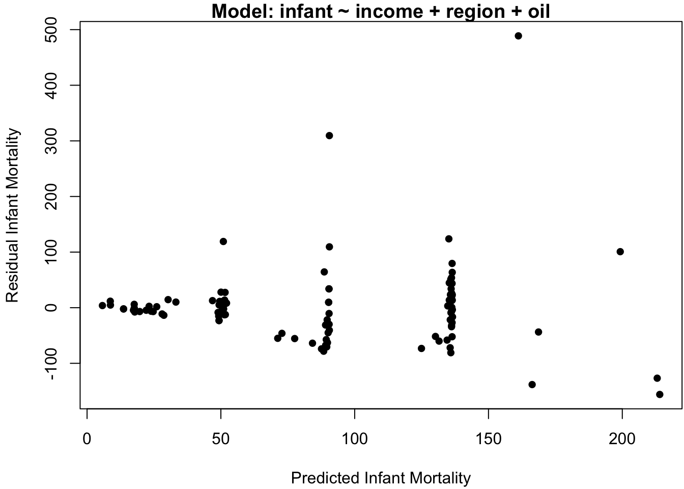

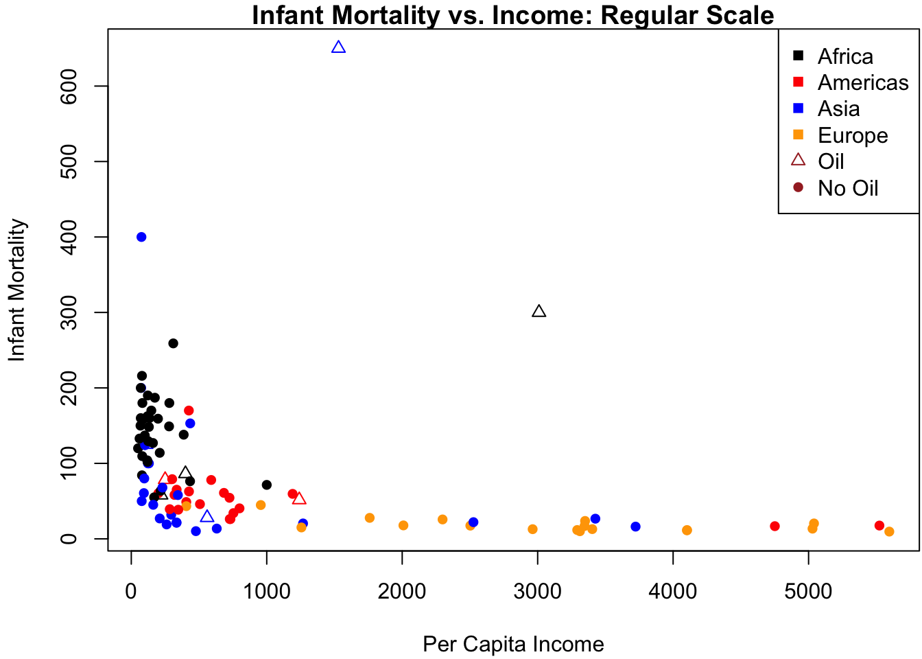
$Data analysis on the original scale. (a) Residuals vs.\ predicted values. (b) Infant mortality vs. income.$ $Data analysis on the original scale. (a) Residuals vs.\ predicted values. (b) Infant mortality vs. income.$

Figure 3.4: Data analysis on the original scale. (a) Residuals vs. predicted values. (b) Infant mortality vs. income.

If the model assumption of iid normal errors adequately describes the data, then the residuals should exhibit no specific pattern about the horizontal axis. However, Figure 3.4a indicates two glaring patterns.

The first is that the predicted values seem to cluster into 4-5 distinct categories. This is not in itself problematic: since the effect of the continuous covariate income is small, we expect the predictions to largely be grouped according to the discrete covariates region and oil (if there are no continuous covariates in the model, then there are exactly as many distinct predicted values as there are discrete covariate categories).

The second pattern in Figure 3.4a is that the magnitude of the residuals seems to increase with the predicted values. This is one of the most common pattern of heteroskedasticity in linear modeling.

So far, we have seen additive error models of the form \[ y = \mu(x) + \eps, \qquad \eps \sim [0, \sigma^2]. \] Here, the square brackets indicate the mean and variance of $\eps$, i.e., $\E[\eps] = 0$ and $\var(\eps) = \sigma^2$. Under such a model, we have \[ y \sim [\mu(x), \sigma^2]. \] In contrast, a multiplicative error model is of the form \[ y = \mu(x) \cdot \eps, \qquad \eps \sim [1, \sigma^2]. \] When the error is multiplicative, we have \[ y \sim [\mu(x), \mu(x)^2 \sigma^2], \] such that both the conditional mean and conditional variance of $y$ depend on $\mu(x)$. Fortunately, a simple treatment of multiplicative models is to put an additive model on the log of $y$, such that \[ \log(y) = \mu(x) + \log(\eps) \iff y = \exp\{\mu(x)\} \cdot \eps. \]

In the linear regression context, the multiplicative model we consider is \[\begin{equation} \log(y_i) = \tilde y_i = x_i'\beta + \tilde \eps_i, \qquad \tilde \eps_i \iid \N(0,\sigma^2). \tag{3.10} \end{equation}\] Under such a model, we can easily obtain the MLE of $\beta$, \[ \hat \beta = \ixtx X' \tilde y. \] Similarly we have the unbiased estimate $\hat \sigma^2$, confidence intervals for $\beta$, hypothesis tests using $t$ and $F$ distributions, and so on. All of these directly follow from the usual additive model (3.10) formulated on the log scale. There are, however, two caveats to consider.

Mean Response Estimates. Suppose we wish to estimate $\mu(x) = \E[y \mid x]$ on the regular scale. Then \[ \mu(x) = \E[y \mid x] = \E[ \exp(x'\beta + \tilde \eps) ] = \exp(x'\beta) \cdot \E[ \eps], \] where $\eps = \exp(\tilde \eps)$.

Definition 3.3 Let $Z \sim \N(\mu, \sigma^2)$. Then $Y = \exp(Z)$ is said to have a log-normal distribution. Its pdf is \[ f_Y(y) = \frac{1}{y\sigma\sqrt{2\pi}} \exp\left\{- \frac 1 2 \frac{(\log(y) - \mu)^2}{\sigma^2}\right\}, \] and its mean and variance are \[ \E[Y] = \exp(\mu + \sigma^2/2), \qquad \var(Y) = (\exp(\sigma^2) - 1) \exp(2\mu + \sigma^2). \]

Thus, $\E[\eps] = \exp(\sigma^2/2)$, such that $\E[y \mid x] = \exp(x'\beta + \sigma^2/2)$. Based on data, the usual estimate of the conditional expectation is \[ \hat \mu(x) = \exp(x'\hat\beta + \hat \sigma^2/2). \]
Prediction Intervals. While $\E[x'\hat \beta] = x'\beta$, unfortunately $\hat \mu(x)$ is not an unbiased estimate for $\mu(x) = \E[y \mid x]$. However, suppose that we wish to make a prediction interval for $y_\star$, a new observation at covariate value $x_\star$. By considering the log-scale model (3.10), we can construct a $1-\alpha$ level prediction interval for $\tilde y_\star = \log(y_\star)$ in the usual way: \[ (L, U) = x_\star' \hat \beta \pm q_\alpha s(x_\star), \] where $s(x_\star) = \hat \sigma \sqrt{1 + x_\star' \ixtx x_\star}$, and for $T \sim t_{(n-p)}$, we have $\Pr( \abs T < q_\alpha) = 1-\alpha$. That is $L = L(X, y, x_\star)$ and $U = U(X, y, x_\star)$ are random variables such that \[ \Pr( L < \tilde y_\star < U \mid \theta) = 1-\alpha, \] regardless of the true parameter values $\theta = (\beta, \sigma)$. But since $\exp(\cdot)$ is a monotone increasing function, \[ \Pr( L < \tilde y_\star < U \mid \theta) = \Pr( \exp(L) < y_\star < \exp(U) \mid \theta), \] such that $(\exp(L), \exp(U))$ is a $1-\alpha$ level prediction interval for $y_\star$.

Let’s return to the Leinhardt dataset. A scatterplot of the data is displayed in Figure 3.4b with different symbols for the points according to region and oil.

# scatterplot on regular scale
clrs <- c("black", "red", "blue", "orange") # different colors for region
pt.col <- clrs[as.numeric(Leinhardt$region)]
symb <- c(16, 2) # different symbols for oil
pt.symb <- c(16, 2)[(Leinhardt$oil=="yes")+1]
plot(Leinhardt$income, Leinhardt$infant,
     pch = pt.symb, col = pt.col,
     xlab = "Per Capita Income", ylab = "Infant Mortality",
     main = "Infant Mortality vs. Income: Regular Scale") # plot title
legend("topright", legend = c(levels(Leinhardt$region), "Oil", "No Oil"),
       pch = c(rep(15, nlevels(Leinhardt$region)), 2, 16),
       col = c(clrs, "brown", "brown")) # legend

Figure 3.4b shows why a linear relation between infant and income clearly fails: the data are highly skewed to the right on each of these axes. Since both variables are also constrained to be positive, there is a good chance that taking logs can “spread out” the values near zero. Indeed, Figure 3.5b changes the axes of Figure 3.4b to the log-scale by adding a log argument to the plot:

plot(Leinhardt$income, Leinhardt$infant,
     log = "xy", # draw x and y axis on log scale
     pch = pt.symb, col = pt.col,
     xlab = "Per Capita Income", ylab = "Infant Mortality",
     main = "Infant Mortality vs. Income: Log Scale") # plot title
legend("topright", legend = c(levels(Leinhardt$region), "Oil", "No Oil"),
       pch = c(rep(15, nlevels(Leinhardt$region)), 2, 16),
       col = c(clrs, "brown", "brown")) # legend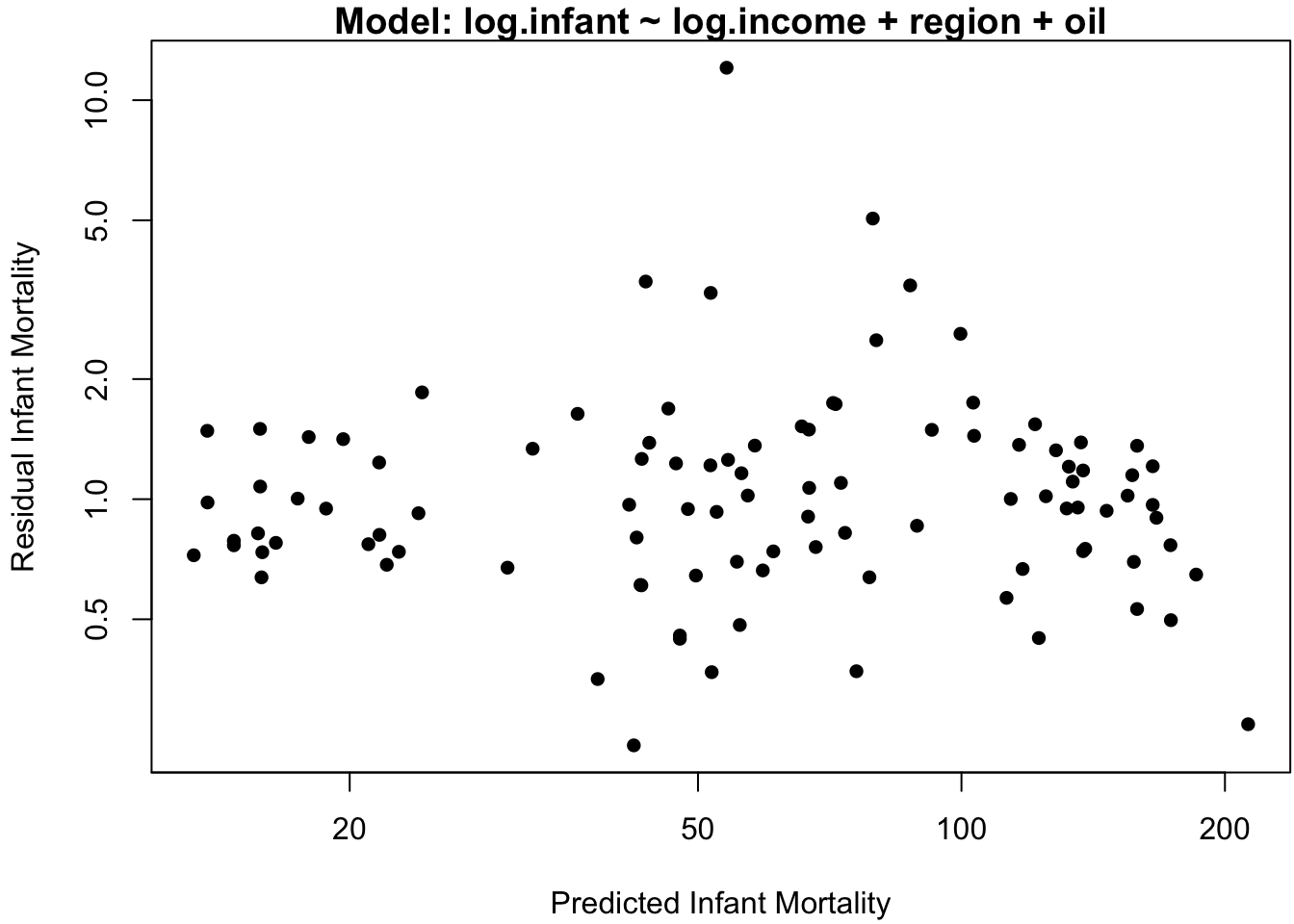

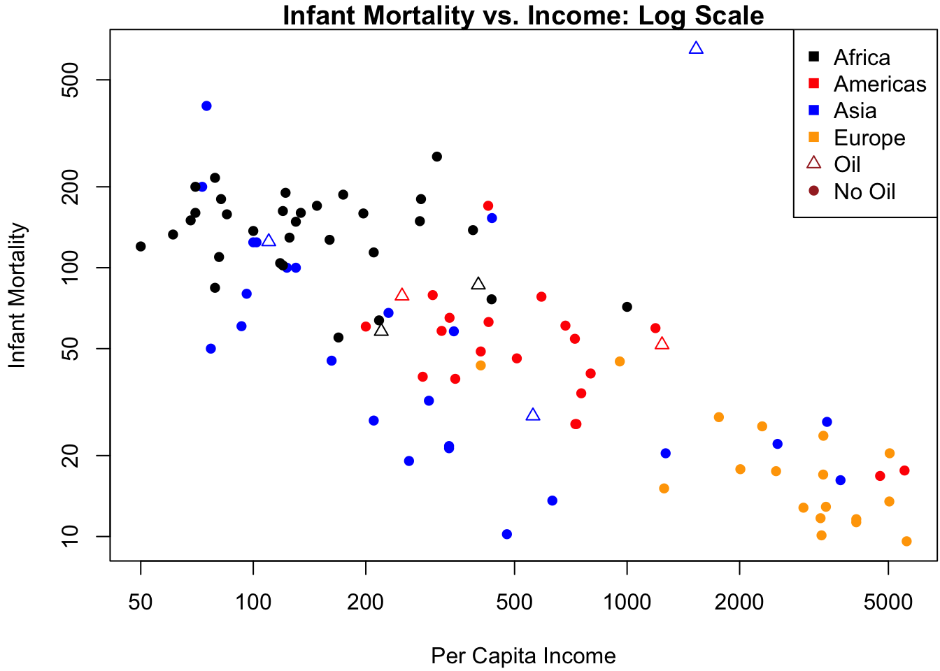
$Data analysis on the log scale. (a) Residuals vs.\ predicted values. (b) Infant mortality vs.\ income.$ $Data analysis on the log scale. (a) Residuals vs.\ predicted values. (b) Infant mortality vs.\ income.$

Figure 3.5: Data analysis on the log scale. (a) Residuals vs. predicted values. (b) Infant mortality vs. income.

The relationship between $\log(\mtt{infant})$ and $\log(\mtt{income})$ is far closer to linear, so we fit the log-log model in $\R$ as follows:

# fit the regression model on the log-log scale
Ml <- lm(I(log(infant)) ~ I(log(income)) + region, data = Leinhardt)
# alternatively, append the transformed variables to the data.frame
Leinhardt$log.infant <- log(Leinhardt$infant)
Leinhardt$log.income <- log(Leinhardt$income)
Ml <- lm(log.infant ~ log.income + region, data = Leinhardt)
coef(summary(Ml)) # coefficient table only

##                  Estimate Std. Error   t value     Pr(>|t|)
## (Intercept)     6.4030058  0.3582859 17.871220 2.685506e-32
## log.income     -0.2993903  0.0674082 -4.441453 2.391601e-05
## regionAmericas -0.6022331  0.1902305 -3.165808 2.072891e-03
## regionAsia     -0.7233423  0.1632444 -4.431038 2.489449e-05
## regionEurope   -1.2028161  0.2588107 -4.647474 1.070092e-05

The residual plot in Figure 3.5a does not indicate egregious departures from homoskedasticity, and the analysis of the $\R$ output confirms a highly significant slope coefficient of log-per-capita income on the log-infant mortality rate.

$\R$ code to produce Figure 3.5a:

# use logarithmic axes so that axis units are intepretable
plot(exp(predict(Ml)), exp(resid(Ml)), # predictions were on log scale
     log = "xy", # axes on logarithmic scale
     main = paste(c("Model:",
       as.character(formula(Ml))[c(2,1,3)]), collapse = " "), # model name
     xlab = "Predicted Infant Mortality",
     ylab = "Residual Infant Mortality", pch = 16)
clrs <- c("black", "red", "blue", "orange") # region colors