5 Model Selection

5.1 Basic Principles of Model Selection

Consider the following problem. Suppose that $y_i \iid f_0(y)$ are iid observations from some true yet unknown distribution $f_0(y)$. We have two candidate models for the data, \[ M_1: \ y_i \iid f_1(y), \qquad M_2: \ y_i \iid f_2(y). \] The question is: based on a given dataset $Y = (\rv y n)$, how to select one of the two candidate models $M_1$ or $M_2$?

It turns out that when both models $f_1(y)$ and $f_2(y)$ as above are fully specified (i.e., no parameters to estimate), then all information in the data about model selection is contained in the likelihood ratio statistic, \[ \lrt = \lrt(Y) = \frac{\prod_{i=1}^n f_1(y_i)}{\prod_{i=1}^n f_2(y_i)}. \] Larger values of $\lrt$ favor model $M_1$ and smaller values favor $M_2$. Thus, the problem of model selection reduces to picking a cutoff value $C$, and selecting $M_1$ if $\lrt > C$ and $M_2$ otherwise. Thus, the question reduces to picking a cutoff value of $C$. This is illustrated in Figure 5.1 with models \[ M_1: y_i \iid \N(5, 1), \qquad M_2: y_i \iid \chi^2_{(3)}, \] and a single observation $n = 1$.

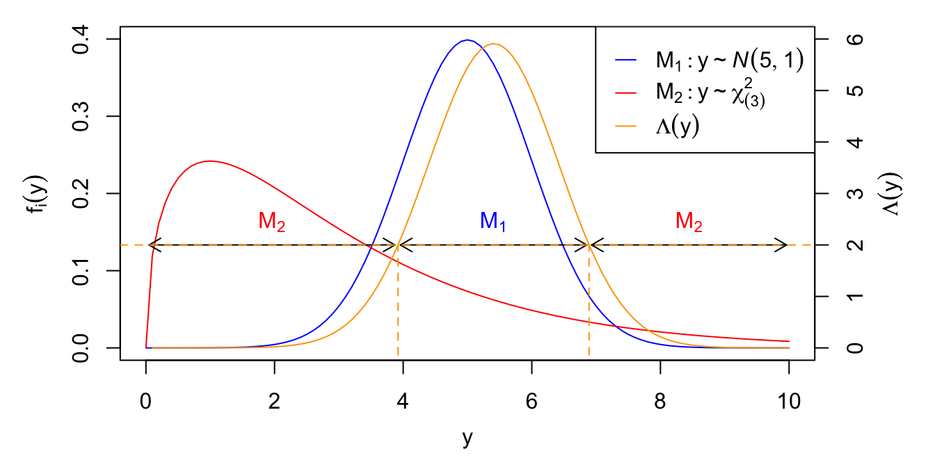
$Model selection based on likelihood ratio statistic. *Left axis:* PDF under models $M_1$ and $M_2$. *Right axis:* Likelihood ratio statistic $\lrt(y) = f_1(y)/f_2(y)$. The horizontal dashed line indicates the cutoff value $C = 2$, for which $M_1$ is selected when $\lrt > C$, and $M_2$ is selected otherwise.$

Figure 5.1: Model selection based on likelihood ratio statistic. Left axis: PDF under models $M_1$ and $M_2$. Right axis: Likelihood ratio statistic $\lrt(y) = f_1(y)/f_2(y)$. The horizontal dashed line indicates the cutoff value $C = 2$, for which $M_1$ is selected when $\lrt > C$, and $M_2$ is selected otherwise.

5.1.1 Choice of Cutoff Value

When there is no preference for either model, a natural choice of cutoff value is $C=1$. Otherwise, if there is a preference for e.g., $M_1$, then we can frame the problem as a hypothesis test, \[ H_0: \tx{$M_1$ is true model} \qquad \iff \qquad H_0: y_i \iid f_1(y), \] and choose $C$ to obtain a given Type-I error rate $\alpha$, \[ \alpha = \Pr(\tx{Pick wrong model} \mid \tx{$M_1$ is true model}) = \Pr(\lrt < C \mid H_0). \]

In the hypothesis testing setting, the likelihood ratio statistic $\lrt$ is optimal in the following sense. Suppose that $T$ is any model selection test statistic for which large values favor model $M_1$, with $T$ and $\lrt$ both calibrated to have the same Type-I error rate $\alpha$. In other words, we have $C_\lrt$ and $C_T$ such that \[ \Pr(\lrt < C_\lrt \mid H_0) = \Pr(T < C_T \mid H_0) = \alpha. \] Consider now the alternative hypothesis \[ H_A: \tx{$M_2$ is true model} \qquad \iff \qquad H_A: y_i \iid f_2(y), \] and define the Type-II error rate $\beta$ as \[ \beta = \Pr(\tx{Pick wrong model} \mid \tx{$M_2$ is true model}). \] Then the optimality result states that \[ \Pr(\lrt > C_\lrt \mid H_A) < \Pr(T > C_T \mid H_A). \] In other words, $\lrt$ has the smallest Type-II error rate among all test statistics having fixed Type-I error rate $\alpha$.

5.1.2 The Estimation Problem

The likelihood ratio statistic $\lrt$ is optimal when $M_1$ and $M_2$ are completely specified. However, this is rarely the case in practice, where we are typically comparing model families \[ M_1: \ y_i \iid f_1(y \mid \theta_1), \qquad M_2: \ y_i \iid f_2(y \mid \theta_2), \] where $\theta_1$ and $\theta_2$ are unknown parameters which need to be estimated from the data. For example, we could have $M_1: y_i \iid \N(\mu, \sigma^2)$ and $M_2 : y_2 \iid \chi^2_{(\nu)}$. One strategy is to adjust the likelihood ratio statistic by considering the most likely parameter values for each model: \[ \lrt = \lrt(Y) = \frac{\max_{\theta_1} \prod_{i=1}^n f_1(y_i \mid \theta_1)}{\max_{\theta_2} \prod_{i=1}^n f_2(y_i \mid \theta_2)} = \frac{\prod_{i=1}^n f_1(y_i \mid \hat \theta_1)}{\prod_{i=1}^n f_2(y_i \mid \hat\theta_2)}, \] where $\hat \theta_1$ and $\hat \theta_2$ are the MLEs for each model. However, this approach is sometimes quite misleading, as seen in the following example.

Example 5.1 Suppose we have a response variable $y$ and a single covariate $x$, and we are choosing between the regression models \[ M_1: y_i \ind \N(\beta_0 + \beta_1 x_i, \sigma^2), \qquad \textstyle M_2: y_i \ind \N\big(\sumi[k] 2 {12} \beta_k \sin(k x_i), \sigma^2\big). \] As an exercise, we can show that the likelihood ratio statistic for any two regression models $M_k: y \sim \N(X\lp k \beta\lp k, \sigma^2)$ is \[ \lrt = \left(\frac{e'\lp 2 e \lp 2}{e'\lp 1 e\lp 1}\right)^{n/2}, \] where $e\lp k = y - X\lp k \hat \beta\lp k$ is the residual vector for model $M_k$. In other words, the likelihood ratio statistic favors the model having smaller residual sum of squares.

Figure 5.2 displays the fit of each model to a dataset of $n = 20$ observations generated from $M_0: y_i \ind \N(\exp(x_i), 4)$.

$Comparison between estimates of the conditional mean $E[y \mid x]$ for models $M_1$ and $M_2$.$

Figure 5.2: Comparison between estimates of the conditional mean $E[y \mid x]$ for models $M_1$ and $M_2$.

The fitted mean of the polynomial model $M_2$ is closer to almost all the data points than that of the linear model $M_1$, so $\lrt \ll 1$. However, the highly nonlinear fitted mean of $M_2$ is hardly any closer than the linear fit of $M_1$ to the true mean under $M_0$. Moreover, the fitted mean under $M_2$ is extremely sensitive to this specific set of $n = 20$ observations. If we obtained a new set of observations, it is likely that we would obtain a completely different nonlinear fit, particularly on the left side of Figure 5.2.

5.1.3 Elements of a Good Model

Suppose that $M_0: y_i \iid f_0(y)$ is the true data-generating process (DGP) and $M: y_i \iid f(y \mid \theta)$ is a candidate model family with unknown parameters $\theta$. A good model $M$ might have some of the following aspects:

Flexibility to capture the true DGP. In other words, there is some $\theta_0$ such that $f(y \mid \theta_0$ is close to $f_0(y)$.
Fitting versus overfitting. Since $\theta$ is unknown, it must be estimated from the data, e.g., using the MLE

\[ \hat \theta = \argmax_{\theta} \mathcal L(\theta \mid Y) = \argmax_{\theta} \prod_{i=1}^n f(y_i \mid \theta). \]

A model is said to fit the data well if $\mathcal L(\hat \theta \mid Y)$ is large (typically in comparison with other models). A model is said to overfit the data if it fits the data, but the estimated distribution $f(y \mid \hat \theta)$ is not close to the true DGP $f_0(y)$. This is the case in Example 5.1: model

\[ \textstyle M_2: y_i \ind \N\big(\sumi[k] 2 {12} \beta_k \sin(k x_i), \sigma^2\big) \]

is too flexible in $\beta = (\rv [2] \beta {12})$, and thus the MLE $\hat \beta$ is highly sensitive to the specific dataset $y = (\rv y n)$. If we get a new dataset, we get a completely different estimate of the conditional mean $\E[y \mid x, \beta = \hat \beta]$. In the context of estimating a conditional distribution $f_0(y \mid x)$ (such as in the regression setting), fitting and overfitting are also referred to as in-sample and out-of-sample predictions.

Explanatory versus predictive power. Suppose we are comparing two regression models

\[ \textstyle M_1: y_i \ind \N\left(\sumi [j] 1 p \beta_j x_{ij}, \sigma^2\right), \qquad M_2: y_i \ind \N\left(\sumi [j] 1 p \sumi [k] 1 r \beta_{jk} x_{ij}^k, \sigma^2\right). \]

Suppose furthermore that model $M_2$ fits the data better than $M_1$ and produces slightly better out-of-sample predictions (we’ll see how to assess this momentarily). While $M_2$ clearly has an edge in terms of predictions, the regression coefficients in $M_1$ have a natural interpretation: $\beta_j$ is the difference in the expectation of $y$ for a unit change in $x_j$ with all other covariates being fixed. On the other hand, what is the meaning in $M_2$ of coefficient $\beta_{j5}$? If the predictive difference between the models is small, in some circumstances one may arguably retain the simpler and more interpretable model $M_1$.

Computational complexity. Some models for financial data are based on differential equations which can take hours or even days to produce the MLE. On the other hand, the $\tx{AR}(p)$ models we saw in the exercises take less than a second to fit, and for all but extreme periods of market instability, both models produce very similar results.

In this course we will only consider the trade-off between points 1 and 2.

5.2 Automated Model Section

Suppose that we have a response $y$ and potential covariates $\rv x Q$ that could enter a linear model. Here, the $x_i$ could be nonlinear terms such as $x_2^2$ or $\log(x_3+1)$, interaction effects such as $x_1 x_4$, or even the set of indicators corresponding to a set of categorical variables, such as $\{I(x_5 = B), I(x_5 = C), I(x_5 = D)\}$. For $Q$ covariates, we may consider the set of $2^Q$ potential models in which any of the covariates may be present or absent from the model. Even for a relatively small set of covariates, this number may be extremely large. For example, suppose we have $p$ continuous covariates and $Q = 2p + p(p-1)/2$ main effects, quadratic terms and interactions. With $p = 7$ main effects, we have $Q = 35$ and $2^Q \approx 34$ billion potential models. Automated model selection can help to narrow down this enormous number to a few reasonable candidate model for closer inspection.

5.2.1 Forward Selection

Start with a base model $M_0: y \sim 1$ corresponding to no covariates, i.e., only the intercept.

Fit all $Q$ models with a single covariate: $M_1: y \sim 1 + x_j$ for $1 \le j \le Q$. Of these $Q$ models, pick the one with the smallest $p$-value of the $F$-test for the significance of $x_j$ in the presence of the intercept. Suppose that this corresponds to $x_k$, which from now on we refer to as $v_1$.
If the $p$-value for $v_1$ is greater than some pre-specified level $\alpha$ (e.g., $\alpha = 0.05$), then forward selection determines that no covariates are significant, so the final model is $M_0: y \sim 1$. Otherwise, the new base model becomes $M_1: y \sim 1 + v_1$.
If the $p$-value for $v_1$ was less than $\alpha$, fit all $Q-1$ models that include $v_1$ and any of the other predictors: $M_2: y \sim 1 + v_1 + x_j$, for $j \neq k$. Let $v_2$ denote the most significant covariate in the presence of $v_1$ and the intercept.
If the $p$-value for $v_2$ is more than $\alpha$, the algorithm returns $M_1$. Otherwise, the new base model becomes $M_2: y \sim 1 + v_1 + v_2$ and we look for the most significant of the $Q-2$ remaining covariates in the presence of $v_1$ and $v_2$.
Forward selection keeps adding variables in this fashion until no new variables are found to be significant in the presence of the current set.

5.2.2 Backward Elimination

Start with a base model $M_Q: y \sim 1 + x_1 + \cdots + x_Q$, which contains all the potential covariates and the intercept.
Find the least significant covariate in $M_Q$. If all covariates are continuous or 2-category factors, then this just means finding the highest $p$-value in the printout of summary(MQ). If there are factors with more than 2 categories, the significance of those covariates in the presence of all the others needs to be calculated with an $F$-test.
If the least significant factor has a $p$-value less than $\alpha$, then all covariates are found to be significant and backward selection returns model $M_Q$. Otherwise, the least significant covariate is dropped from the model and we look for the least significant of the remaining $Q-1$ (always in the presence of all other covariates in the model).
Backward selection keeps dropping terms from the base model $M_Q$ until all remaining covariates are significant at level $\alpha$.

5.2.3 Stepwise Selection

The algorithms above don’t necessarily produce the same results. In general, backward elimination tends to perform better than forward selection for the following reason. Suppose that we have three covariates $x_1$, $x_2$ and $x_3$. It might well be that the best combination of these covariates is $y \sim 1 + x_2 + x_3$, but that the most significant covariate in the presence of only the intercept is $x_1$. Then, $x_1$ would be added at the first stage by forward selection and necessarily included in the final model.

On the other hand, it could easily be that $Q > n$ (imagine including all main effects, interactions, and quadratic terms into a model), in which case the parameters of the base model for backward elimination cannot be estimated by the usual formula, as $X'X$ is no longer invertible.

Stepwise selection is a compromise between the two approaches which can add or drop a variable at any stage.

Given a minimum model $M_0$ (usually just the intercept) and the maximal model $M_Q$ which includes all terms, start with a base model $M_B$ somewhere between the two (I usually start with the model containing only main effects).
Find the most significant covariate and add it if its $p$-value is below $\alpha_\tx{add}$.
Find the least significant covariate and delete it if its $p$-value is above $\alpha_\tx{drop}$.
Continue in this manner until no further covariates can be added or dropped.

With stepwise selection, covariates may thus enter and leave the model more than once.

5.2.4 Illustration

Automatic model selection can be carried out with using the step function. To illustrate, let us revisit the dataset which contains 600 observations from a very large study of students in the U.S. carried out in 1980 by the National Center for Education in Statistics. The variables of interest in the dataset are:

math: Standardized math test scores.
gender: Gender as male or female.
lang: First language, with levels english, spanish, mandarin.
minor: Identify as an ethnic minority yes or no.
ses: Socio-economic status, with levels low, middle, high.
sch: High school type, with levels public, private.
prog: High school program, with levels general, academic, vocation.
career: Career plan, a categorical covariate with 17 levels (the code below shows how to display them all).
locus: Locus of control, a continuous covariate indicating the subject’s self-perceived degree of control over the events which affect them (higher = more perceived control).
concept: Self-concept, a continuous covariate reflecting the subject’s self-perceived academic abilities (higher = more self-perceived ability).
mot: Motivation, a continuous covariate (higher = more self-perceived motivation).

# high school and beyond dataset
hsb <- read.csv("HSB2.csv")
hsbm <- hsb[c(13, 1:6, 10, 7:9)] # keep only variables listed above

summary(hsbm) # summary statistics

##       math          gender              lang               ses           
##  Min.   :31.80   Length:600         Length:600         Length:600        
##  1st Qu.:44.50   Class :character   Class :character   Class :character  
##  Median :51.30   Mode  :character   Mode  :character   Mode  :character  
##  Mean   :51.85                                                           
##  3rd Qu.:58.38                                                           
##  Max.   :75.50                                                           
##     minor               sch                prog              career         
##  Length:600         Length:600         Length:600         Length:600        
##  Class :character   Class :character   Class :character   Class :character  
##  Mode  :character   Mode  :character   Mode  :character   Mode  :character  
##                                                                             
##                                                                             
##                                                                             
##      locus             concept               mot        
##  Min.   :-2.23000   Min.   :-2.620000   Min.   :0.0000  
##  1st Qu.:-0.37250   1st Qu.:-0.300000   1st Qu.:0.3300  
##  Median : 0.21000   Median : 0.030000   Median :0.6700  
##  Mean   : 0.09653   Mean   : 0.004917   Mean   :0.6608  
##  3rd Qu.: 0.51000   3rd Qu.: 0.440000   3rd Qu.:1.0000  
##  Max.   : 1.36000   Max.   : 1.190000   Max.   :1.0000

table(hsbm$career) # full breakdown for categorical variable "career"

## 
##    clerical   craftsman      farmer   homemaker     laborer     manager 
##          50          39          11          33          12          23 
##    military not working   operative       prof1       prof2  proprietor 
##          19           9          24         161          94          22 
##  protective       sales      school     service   technical 
##           9          12          17          29          36

In order to perform automated model selection, we need to pick a minimal, maximal, and starting point model. The minimal model is usually taken to be only the intercept:

M0 <- lm(math ~ 1, data = hsbm) # minimal model: intercept only

A default value for the maximal model is often to just include all the main effects and interactions:

Mmax <- lm(math ~ (.)^2, data = hsbm) # all main effects and interactions

However, this maximal model has 284 coefficients, many of which are NA:

# find model coefficients which are NA
beta.max <- coef(Mmax)
names(beta.max)[is.na(beta.max)]

##  [1] "gendermale:careerprotective"    "langmandarin:minoryes"         
##  [3] "langspanish:minoryes"           "langmandarin:careerfarmer"     
##  [5] "langspanish:careerfarmer"       "langmandarin:careerhomemaker"  
##  [7] "langspanish:careerlaborer"      "langmandarin:careermanager"    
##  [9] "langmandarin:careernot working" "langspanish:careernot working" 
## [11] "langmandarin:careerproprietor"  "langmandarin:careerprotective" 
## [13] "langmandarin:careersales"       "langmandarin:careerschool"     
## [15] "langspanish:careerschool"       "langmandarin:careerservice"    
## [17] "sesmiddle:careerfarmer"         "sesmiddle:careerlaborer"       
## [19] "sesmiddle:careeroperative"      "minoryes:careerfarmer"         
## [21] "minoryes:careersales"           "schpublic:careerfarmer"        
## [23] "schpublic:careernot working"    "progvocation:careerlaborer"    
## [25] "proggeneral:careerprotective"   "careernot working:mot"         
## [27] "careerprotective:mot"

To investigate the cause for these missing coefficient estimates, we can use the table function to cross-tabulate the number of students between some of the pairs of covariates listed above:

# number of respondents in minor and lang covariates
table(hsbm[c("minor", "lang")])

##      lang
## minor english mandarin spanish
##   no      437        0       0
##   yes      58       34      71

Thus we see that none of the first language English speaking respondents identified as minorities. Table 5.1 displays the columns of the design matrix corresponding to only the categorical variables lang and minor.

langminor <- data.frame(
  lang = rep(c("E", "M", "S"), times = 2),
  minor = rep(c("N", "Y"), each = 3),
  `(Intercept)` = rep(1, 6),
  langM = c(0, 1, 0, 0, 1, 0),
  langS = c(0, 0, 1, 0, 0, 1),
  minorY = c(0, 0, 0, 1, 1, 1),
  `langM:minorY` = c(0, 0, 0, 0, 1, 0),
  `langS:minorY` = c(0, 0, 0, 0, 0, 1)
)
kableExtra::kbl(langminor,
                caption = "Design matrix for main effects and interactions between `lang` and `minor`.  Only the relevant rows and columns of the full design matrix are shown.")

Table 5.1: Design matrix for main effects and interactions between `lang` and `minor`. Only the relevant rows and columns of the full design matrix are shown.
lang	minor	X.Intercept.	langM	langS	minorY	langM.minorY	langS.minorY
E	N	1	0	0	0	0	0
M	N	1	1	0	0	0	0
S	N	1	0	1	0	0	0
E	Y	1	0	0	1	0	0
M	Y	1	1	0	1	1	0
S	Y	1	0	1	1	0	1

Since the data contains no respondents with lang=mandarin and minor=no, there is no one in the dataset corresponding to the second row of the matrix in Table 5.1. Thus, column langM and langM:minorY are exactly the same. This must also be true for the corresponding columns of the design matrix of Mmax, since they are just duplicated values of the rows in Table 5.1. In other words, the design matrix in Mmax has linearly dependent columns, and thus a unique MLE of $\beta$ does not exist. handles this case by reporting NA for the interaction term.

This situation is typical for models containing interactions between categorical covariates having many levels. To avoid fitting problems, let’s consider a slightly smaller model, namely:

No interaction between lang and minor.
No interactions between the 17-level categorical variable career and anything else, but keep career as a main effect.
Add quadratic terms for the continuous covariates locus, concept, and mot.

This new maximal model is coded in as:

# new maximal model
Mmax <- lm(math ~ (.-career)^2 + career - lang:minor +
              I(locus^2) + I(concept^2) + I(mot^2),
            data= hsbm)
anyNA(coef(Mmax)) # check if there are any remaining NAs

## [1] FALSE

Finally, for stepwise selection we also need to specify a starting point model. A common choice for this is the model with main effects only:

Mstart <- lm(math ~ ., data = hsbm) # starting model for stepwise selection

We now run each of the three algorithms for automated model selection as implemented in :

# forward selection
system.time({ # time the calculation
  Mfwd <- step(object = M0, # starting point model
               scope = list(lower = M0, upper = Mmax), # smallest and largest model
               direction = "forward",
               trace = FALSE) # trace prints out information
})

##    user  system elapsed 
##   0.219   0.019   0.238

# backward elimiation
system.time({
  Mback <- step(object = Mmax, # starting point model
                scope = list(lower = M0, upper = Mmax),
                direction = "backward", trace = FALSE)
})

##    user  system elapsed 
##   1.572   0.126   1.699

# stepwise selection (both directions)
system.time({
  Mstep <- step(object = Mstart,
                scope = list(lower = M0, upper = Mmax),
                direction = "both", trace = FALSE)
})

##    user  system elapsed 
##   0.327   0.036   0.363

# number of parameters in each model
c(fwd = length(coef(Mfwd)), back = length(coef(Mback)), step = length(coef(Mstep)))

##  fwd back step 
##   21   29   24

The first thing we notice is that forward selection is the fastest calculation, backward elimination is the slowest, and stepwise is somewhere between the two. This is because backward elimination is starting with more covariates, such that $\ixtx$ takes more time to calculate.

The next thing to notice is that forward selection has the least number of coefficients, backward elimination has the most, and stepwise is somewhere between the two. This is a relatively common pattern, in that forward selection is greedier in including marginally significant covariates. That is, suppose we have $Q = 3$, and $y \sim x_1$ is the best one-term model. If $y \sim x_2 + x_3$ is the best two-term model, then forward selection has no hope of achieving it.

Finally, let’s check if any of the models are nested within each other, i.e., the covariates of $M_1$ are a subset of those in $M_2$. If this is the case, then we can choose between $M_1$ and $M_2$ by setting $H_0: M_1$ and using an $F$-test on the extra covariates of $M_2$ being equal to zero.

# display covariates in each model
Mfwd$call

## lm(formula = math ~ prog + lang + minor + locus + ses + I(mot^2) + 
##     gender + concept + minor:ses + lang:gender + minor:gender + 
##     lang:concept + prog:gender, data = hsbm)

Mback$call

## lm(formula = math ~ gender + lang + ses + minor + sch + prog + 
##     locus + concept + I(mot^2) + gender:lang + gender:minor + 
##     gender:prog + lang:sch + lang:concept + ses:sch + ses:concept + 
##     minor:prog + sch:locus, data = hsbm)

Mstep$call

## lm(formula = math ~ gender + lang + ses + minor + sch + prog + 
##     locus + concept + mot + ses:sch + lang:concept + minor:sch + 
##     gender:lang + gender:minor + sch:locus + gender:prog, data = hsbm)

We see that the term minor:ses is present in Mfwd but not Mback, and conversely, ses:sch is present in Mback but not in Mfwd. Therefore, we can’t use an $F$-test to compare these models. So what should we do?

5.3 Manual Model Selection

In the previous example, we saw how to reduce a very large number number of potential models to just a few interesting candidates that should be compared more carefully. Here we shall see how to make such case-by-case comparisons.

5.3.1 Cross-Validation

We saw that the likelihood ratio statistic \[ \lrt = \frac{\prod_{i=1}^n f_1(y_i \mid \hat \theta_1)}{\prod_{i=1}^n f_2(y_i \mid \hat\theta_2)} \] tends to favor models that overfit the data, i.e., produce very large likelihoods $\prod_{i=1}^n f_k(y_i \mid \hat \theta_k)$ at the MLE $\hat \theta_k$, without the estimated data distribution $f_k(y \mid \hat \theta_k)$ being close to the true distribution $f_0(y)$. To mitigate this problem, cross-validation divides the $n$ observations into disjoint “training” and “testing” subsets, \[\begin{equation} \St_\train \cup \St_\test = \{1,\ldots,n\}, \qquad \St_\train \cap \St_\test = \emptyset. \tag{5.1} \end{equation}\] Then, it uses the training (or calibration) set $\St_\train$ to estimate $\theta_k$ and the testing (or validation) set $\St_\test$ to calculate $\lrt$. More specifically:

Randomly divide the $n$ observations into training and testing subsets as in (5.1).
Calculate the training set MLEs

\[ \hat \theta_k^\train = \argmax_{\theta_k} \sum_{i \in \St_\train} \log f_k(y_i \mid\theta_j). \]
Calculate the desired model selection metric on the test set. Two of the most common examples of these are:
- The out-of-sample likelihood ratio statistic:
  
  \[ \lrt^\test = \frac{\prod_{i \in \St_\test} f_1(y_i \mid \hat \theta_1^\train)}{\prod_{i \in \St_\test} f_2(y_i \mid \hat \theta_2^\train)}. \]
- The mean square prediction error (MSPE): When estimating conditional distributions of the form $M_k: f_k(y \mid x, \theta_k)$, the MSPE for model $M_k$ is given by
  
  \[ \mspe_k = \sum_{i \in \St_\test} \left(y_i - \E[y \mid x = x_i, \theta_k = \hat \theta_k^\train]\right)^2. \]
  
  For linear regression models, this boils down to
  
  \[ \mspe_k = \sum_{i \in \St_\test} \left(y_i - x_i' \hat \beta_k^\train\right)^2. \]

Repeat steps 1-3 many times to avoid a single bad randomization of $\St_\train$ and $\St_\test$ biasing results. Usually about 1000 times starts to give a clear picture.

Figure 5.3 displays the square root of the MSPE (which has units of response) and the histogram of the out-of-sample likelihood ratio statistic for a cross-validation comparison between models Mfwd and Mstep. The difference between models is very small, but there is a slight preference for the richer model Mstep.

# models to compare
M1 <- Mfwd
M2 <- Mstep
Mnames <- expression(M[FWD], M[STEP])

# Cross-validation setup
nreps <- 2e3 # number of replications
ntot <- nrow(hsbm) # total number of observations
ntrain <- 500 # size of training set
ntest <- ntot-ntrain # size of test set
mspe1 <- rep(NA, nreps) # sum-of-square errors for each CV replication
mspe2 <- rep(NA, nreps)
logLambda <- rep(NA, nreps) # log-likelihod ratio statistic for each replication

system.time({
  for(ii in 1:nreps) {
    if(ii%%400 == 0) message("ii = ", ii)
    # randomly select training observations
    train.ind <- sample(ntot, ntrain) # training observations
    # refit the models on the subset of training data; ?update for details!
    M1.cv <- update(M1, subset = train.ind)
    M2.cv <- update(M2, subset = train.ind)
    # out-of-sample residuals for both models
    # that is, testing data - predictions with training parameters
    M1.res <- hsbm$math[-train.ind] -
      predict(M1.cv, newdata = hsbm[-train.ind,])
    M2.res <- hsbm$math[-train.ind] -
      predict(M2.cv, newdata = hsbm[-train.ind,])
    # mean-square prediction errors
    mspe1[ii] <- mean(M1.res^2)
    mspe2[ii] <- mean(M2.res^2)
    # out-of-sample likelihood ratio
    M1.sigma <- sqrt(sum(resid(M1.cv)^2)/ntrain) # MLE of sigma
    M2.sigma <- sqrt(sum(resid(M2.cv)^2)/ntrain)
    # since res = y - pred, dnorm(y, pred, sd) = dnorm(res, 0, sd)
    logLambda[ii] <- sum(dnorm(M1.res, mean = 0, sd = M1.sigma, log = TRUE))
    logLambda[ii] <- logLambda[ii] -
      sum(dnorm(M2.res, mean = 0, sd = M2.sigma, log = TRUE))
  }
})

## ii = 400

## ii = 800

## ii = 1200

## ii = 1600

## ii = 2000

##    user  system elapsed 
##  23.274   0.239  23.540

# plot rMSPE and out-of-sample log(Lambda)
par(mfrow = c(1,2))
par(mar = c(4.5, 4.5, .1, .1))
boxplot(x = list(sqrt(mspe1), sqrt(mspe2)), names = Mnames, cex = .7,
        ylab = expression(sqrt(MSPE)), col = c("yellow", "orange"))
hist(logLambda, breaks = 50, freq = FALSE,
     xlab = expression(Lambda^{test}),
     main = "", cex = .7)
abline(v = mean(logLambda), col = "red") # average value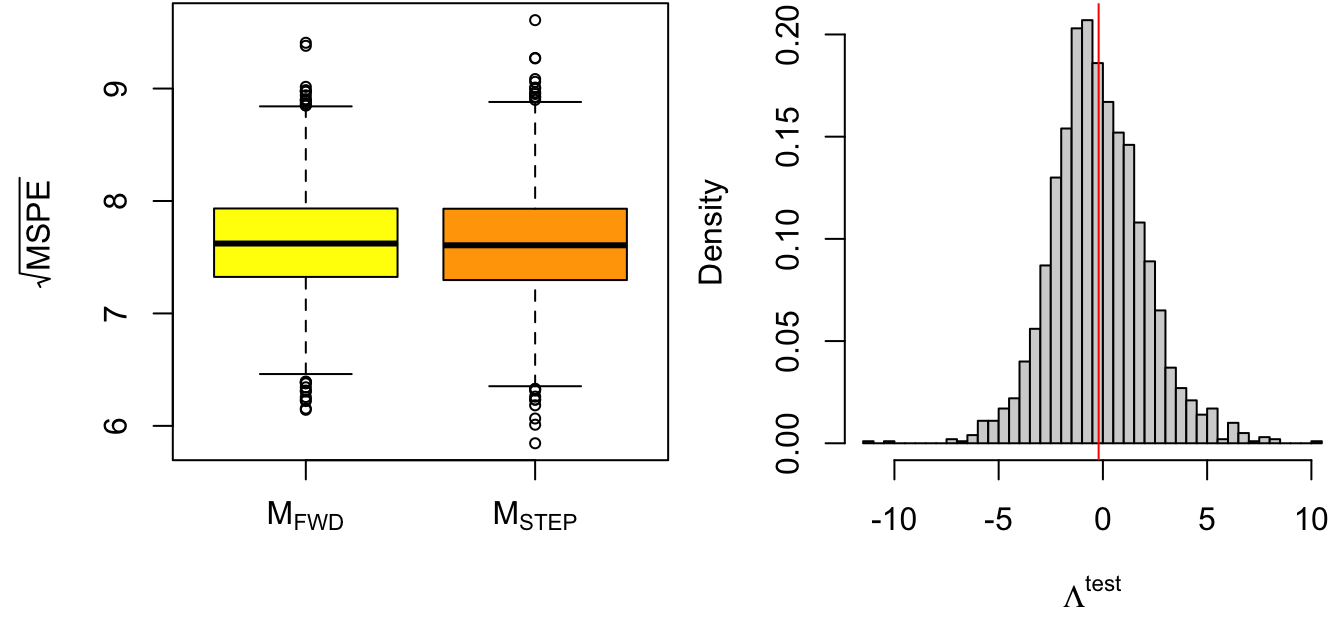

Cross-validation model comparison results. Left: Root mean square prediction error (rMSPE). Right: Out-of-sample likelihood ratio statistic.

Figure 5.3: Cross-validation model comparison results. Left: Root mean square prediction error (rMSPE). Right: Out-of-sample likelihood ratio statistic.

Cross-validation is an excellent approach to model selection, but it does have a couple of caveats:

It’s computationally expensive, since MLEs need to be calculated over and over again.
It’s entirely based on predictive (as opposed to explanatory power). Therefore, with large enough sample sizes, models with more parameters tend to be systematically preferred.
It’s not always clear how to pick the training and testing sample sizes $n_\train$ and $n_\test$. The larger the training sample, the more cross-validation tends to favor more complicated models. On the other hand, when $n_\train$ is too small, then more complicated models tend to overfit the training sample, thus having poor predictive performance on $\St_\test$.

A fundamental problem with model selection in general is that e.g., confidence intervals and p-values calculated in the usual way are incorrect. That is, we know that without model selection, the pivotal quantity $T = (\hat \beta_j - \beta_j)/\se(\hat \beta_j)$ has a $t_{(n-p)}$ distribution, where $p$ is the number of columns of the design matrix $X$. However, when we apply model selection, the number of columns depends on the response variables $y$. In other words, each time we collect a new dataset $y$ we potential obtain a different $X$, and hence a different number of columns $p$. This problem is called post-selection inference and is one of the great open challenges in contemporary statistical research.
As with any statistical method, if the full dataset of $n$ observations is from $M_2$ but by random chance happens to favor $M_1$, then no amount of cross-validation can reverse this result. This is simply a reminder that no statistical method always gives the right answer. However, as $n\to \infty$ the probability of randomly getting a bad dataset becomes less and less likely.

The next two methods present less reliable but much faster approaches to manual model selection.

5.3.2 PRESS Statistics

Note that if we do cross-validation with $n_\test = 1$, then the MSPE is equivalent to the squared PRESS statistic: \[ \tx{PRESS}_i = y_i - \hat y\lp i = y_i - x_i' \hat \beta\lp i = \frac{e_i}{1-h_i}. \] In other words, for regression models with $n_\test = 1$, all $n$ PRESS statistics can be calculated with a single model fit. A fast alternative to cross-validation is thus to select model $M_1$ if \[ \sum_{i=1}^n (\tx{PRESS}_i\sp 1)^2 < \sum_{i=1}^n (\tx{PRESS}_i\sp 2)^2. \]

5.3.3 Akaike Information Criterion

Recall the basic setup for model selection in the presence of unknown parameters: we have some true data-generating process $y_i \iid f_0(y)$, and two candidate models \[ M_1: \ y_i \iid f_1(y \mid \theta_1), \qquad M_2: \ y_i \iid f_2(y \mid \theta_2), \] with parameters $\theta_1$ and $\theta_2$ to be estimated from a given set of observations $Y = (\rv y n)$. We saw that the likelihood ratio statistic \[ \lrt = \frac{\prod_{i=1}^n f_1(y_i \mid \hat \theta_1)}{\prod_{i=1}^n f_2(y_i \mid \hat\theta_2)} \] which picks model $M_1$ or $M_2$ depending on whether $\lrt$ is above or below 1 can have very bad performance if the models are too richly parametrized relative to the number of observations, i.e., overfit the data. The Akaike Information Criterion (AIC) is an adjustment to the likelihood ratio statistic which penalizes overfitting as described below.

Let’s begin with a popular notion of “distance” between distributions. The Kullback-Liebler divergence between the true distribution $f_0(y)$ and a candidate distribution $f(y)$ is defined as \[ \kl_0(f) = \kl_0\big\{f(y)\big\} = \int \log\left(\frac{f_0(y)}{f(y)}\right) \cdot f_0(y) \ud y = E_0\big[\log f_0(y) - \log f(y)\big], \] where the expectation is taken over the true distribution $y \sim f_0(y)$. There are two important properties of the KL divergence that make it appealing for model selection:

It turns out that

\[ \kl_0(f) \ge 0, \qquad \kl_0(f) = 0 \iff f(y) = f_0(y). \]

In other words, the KL divergence between $f(y)$ and $f_0(y)$ attains its unique minimum when $f(y) = f_0(y)$ is the true distribution itself.
Consider a model family $M: y_i \iid f(y \mid \theta) = f_\theta(y)$ parametrized by an unknown $\theta$. In practice, we would commonly be estimating $\theta$ by the MLE, $\hat \theta = \argmax_{\theta} \prod_{i=1}^n f(y \mid \theta)$. Remarkably, it turns out that

\[ \lim_{n\to \infty} \hat \theta = \argmin_{\theta} \kl_0\big\{f(y \mid \theta)\big\}. \] In other words, the distribution $f(y \mid \hat \theta)$ estimated by maximum likelihood converges to the distribution in the model family closest to $f_0(y)$.

Therefore, let \[ \tilde f_k(y) = f_k(y \mid \tilde \theta_k), \qquad \tilde \theta_k = \argmin_{\theta_k} \kl_0\big\{f_k(y \mid \theta_k)\big\} \] denote the “best distribution” in model family $M_k$, in the sense of minimizing the KL diverge to the true model $f_0(y)$. Akaike argues that we ought to pick the model family $M_k$ for which the KL diverges to $f_0(y)$ is smallest, i.e., pick model $M_1$ if \[ \kl_0(\tilde f_1) - \kl_0(\tilde f_2) = E_0\big[\log f_2(y \mid \tilde \theta_2) - \log f_1(y \mid \tilde \theta_1)\big] < 0. \]
The problem thus reduces to estimating the expectations \[ \tau_k = E_0\big[\log f_k(y \mid \tilde \theta_k)\big]. \]

Suppose that the optimal parameter values $\tilde \theta_k$ were known. Then \[ \frac 1 n \sumi 1 n \log f_k(y_i \mid \tilde \theta_k) = g_k(y_i) \] is just an average of iid random variables $z_i = g_k(y_i)$, so by e.g., the Central Limit Theorem we know that the sample mean converges to its expectation, \[ \frac 1 n \sumi 1 n \log f_k(y_i \mid \tilde \theta_k) \to E_0\left[\frac 1 n \sumi 1 n \log f_k(y_i \mid \tilde \theta_k)\right] = E_0\big[\log f_k(y \mid \tilde \theta_k)\big] = \tau_k. \] For $\tilde \theta_k$ unknown, we would replace it by its MLE $\hat \theta_k$. Akaike’s next step was to expand the resulting estimator in terms of increasing powers of $1/n$: \[ \hat \tau_k = \frac 1 n \sumi 1 n \log f_k(y_i \mid \hat \theta_k) = \tau_k + \frac{\dim(\theta_k)}{n} + \frac{c_2}{n^2} + \frac{c_3}{n^3} + \cdots, \] where $\dim(\theta_k)$ is the number of parameters in the model. The Akaike Information Criterion (AIC) is a scaled version of the first-order approximation in this expansion, $\tau_k \approx \hat \tau_k - \dim(\theta_k)/n$: \[ \aic_k = -2 \sum_{i=1}^n \log f_k(y_i \mid \hat \theta_k) + 2\dim(\theta_k), \] and picks $M_1$ over $M_2$ if \[ \aic_2 - \aic_1 > 0 \quad \iff \quad \lrt = \frac{\prod_{i=1}^n f_1(y_i \mid \hat \theta_1)}{\prod_{i=1}^n f_2(y_i \mid \hat \theta_2)} > \exp\big\{\dim(\theta_1) - \dim(\theta_2)\big\} = C. \] If $\dim(\theta_1) = \dim(\theta_2)$, then selecting with AIC is identical to selecting with the likelihood ratio statistic $\lrt$. Otherwise, the AIC penalizes richer models by one unit of $\log(\lrt)$ per additional parameter.

For a linear regression model $y \sim \N(X, \beta)$ with $p$ covariates, we have \[ \aic = n\left(1 + \log(e'e/n) + \log(2\pi)\right) + 2 (p+1). \] The first part is left as an exercise, but the number of parameters in the model is $p+1$ if we include the unknown $\sigma$.

5.3.4 Illustration

The code below calculates the AIC and sum of squared PRESS residuals for models Mfwd and Mback. We can also look at boxplots of the absolute value of the PRESS residuals as in Figure 5.4. In this case, the results are consistent with cross-validation results of Section 5.3.1, i.e., giving a slight predictive advantage to the stepwise selection model Mstep.

# models to compare
M1 <- Mfwd
M2 <- Mstep
Mnames <- expression(M[FWD], M[STEP])

# AIC statistic
# calculate the long way for M1
sig1 <- sqrt(sum(resid(M1)^2)/nrow(hsbm)) # mle divides by n, not n-p
ll1 <- dnorm(hsbm$math, mean = predict(M1), sd = sig1, log = TRUE) # log-pdf
ll1 <- sum(ll1)
p1 <- length(M1$coef)+1 # number of parameters
AIC1 <- -2*ll1 + 2*p1
# calculate the R way
AIC1 - AIC(M1)

## [1] 0

AIC2 <- AIC(M2) # for M2

# PRESS statistics
press1 <- resid(M1)/(1-hatvalues(M1)) # M1
press2 <-  resid(M2)/(1-hatvalues(M2)) # M2

# display results
disp <- rbind(AIC = c(AIC1, AIC2),
              PRESS = c(sum(press1^2), sum(press2^2)))
colnames(disp) <- Mnames
disp # both metrics favor M2

##          M[FWD]  M[STEP]
## AIC    4140.747  4137.21
## PRESS 34786.524 34557.28

# plot PRESS statistics
par(mar = c(3, 6, 1, 1))
boxplot(x = list(abs(press1), abs(press2)), names = Mnames,
        ylab = expression(group("|", PRESS[i], "|")),
        col = c("yellow", "orange"))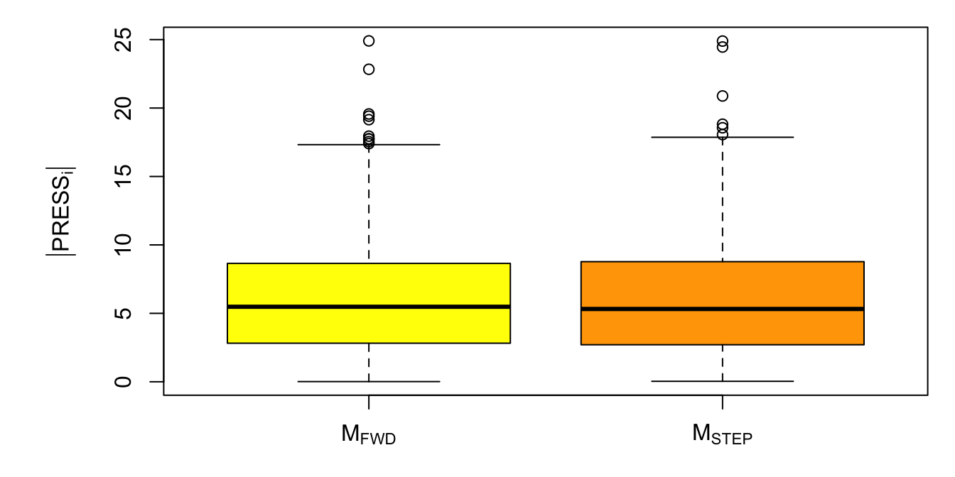

Figure 5.4: Boxplot of squared PRESS statistics for models Mfwd and Mstep.