Loglikelihood for multivariate Ornstein-Uhlenbeck process.

Computes the exact Euler loglikelihood for any amount of missing data using a Kalman filter.

mou.loglik(X, dt, nvar.obs, Gamma, Lambda, Phi, mu0, Sigma0)

Arguments

X	An nobs x ndims matrix of complete data.
dt	A scalar or length nobs-1 vector of interobservations times.
nvar.obs	A scalar or length nobs vector of integers between 0 and ndims denoting the number of observed SDE variables in each row of data. Defaults to ndims. See sde.init() for details.
Gamma	A ndims x ndims of linear-drift parameters. See Details.
Lambda	A length-ndims vector of constant-drift parameters. See Details.
Phi	A ndims x ndims positive definite variance matrix. See Details.
mu0, Sigma0	Mean and variance of marginal multivariate normal distribution of X[1,]. Defaults to iid standard normals for each component.

Value

Scalar value of the loglikelihood. See Details.

Details

The \(p\)-dimensional multivariate Ornstein-Uhlenbeck (mOU) process \(Y_t = (Y_{1t}, \ldots, Y_{dt})\) satisfies the SDE $$ dY_t = (\Gamma Y_t + \Lambda)dt + \Phi^{1/2} dB_t, $$ where \(B_t = (B_{1t}, \ldots, B_{pt})\) is \(p\)-dimensional Brownian motion. Its Euler discretization is of the form $$ Y_{n+1} = Y_n + (\Gamma Y_n + \Lambda) \Delta_n + \Phi^{1/2} \Delta B_n, $$ where \(Y_n = Y(t_n)\), \(\Delta_n = t_{n+1} - t_n\) and $$ \Delta B_n = B(t_{n+1}) - B(t_n) \stackrel{\textnormal{ind}}{\sim} \mathcal N(0, \Delta_n). 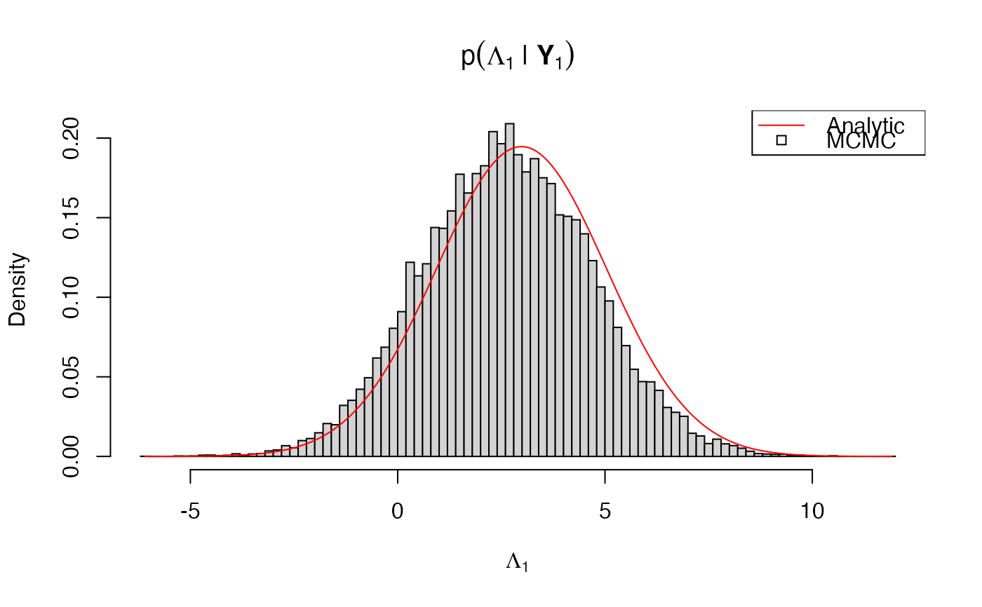$$ Thus, \(Y_0, \ldots, Y_N\) is multivariate normal Markov chain for which the marginal distribution of any subset of timepoints and/or components can be efficiently calculated using the Kalman filter. This can be used to check the MCMC output of sde.post() as in the example.

Examples

# \donttest{
# bivariate OU model
bmod <- sde.examples("biou")

# simulate some data

# true parameter values
Gamma0 <- .1 * crossprod(matrix(rnorm(4),2,2))
Lambda0 <- rnorm(2)
Phi0 <- crossprod(matrix(rnorm(4),2,2))
Psi0 <- chol(Phi0) # precompiled model uses the Cholesky scale
theta0 <- c(Gamma0, Lambda0, Psi0[c(1,3,4)])
names(theta0) <- bmod$param.names
# initial value
Y0 <- rnorm(2)
names(Y0) <- bmod$data.names

# simulation
dT <- runif(1, max = .1) # time step
nObs <- 10
bsim <- sde.sim(bmod, x0 = Y0, theta = theta0,
                dt = dT, dt.sim = dT, nobs = nObs)
#> Number of normal draws required: 10
#> Running simulation...
#> Execution time: 0 seconds.
#> Bad Draws = 0
YObs <- bsim$data

# inference via MCMC
binit <- sde.init(bmod, x = YObs, dt = dT, theta = theta0,
                  nvar.obs = 1) # second component is unobserved
# only Lambda1 is unknown
fixed.params <- rep(TRUE, bmod$nparams)
names(fixed.params) <- bmod$param.names
fixed.params["Lambda1"] <- FALSE
# prior on (Lambda1, Y_0)
hyper <- list(mu = c(0,0), Sigma = diag(2))
names(hyper$mu) <- bmod$data.names
dimnames(hyper$Sigma) <- rep(list(bmod$data.names), 2)

# posterior sampling
nsamples <- 1e5
burn <- 1e3
bpost <- sde.post(bmod, binit, hyper = hyper,
                  fixed.params = fixed.params,
                  nsamples = nsamples, burn = burn)
#> Output size:
#> params = 9e+05
#> data = 40000
#> Running posterior sampler...
#> Execution time: 0.3 seconds.
#> Bridge accept: min = 74.8%, avg = 87.6%
#> Lambda1 accept: 44.2%
#> Y20 accept: 100%
L1.mcmc <- bpost$params[,"Lambda1"]

# analytic posterior
L1.seq <- seq(min(L1.mcmc), max(L1.mcmc), len = 500)
L1.loglik <- sapply(L1.seq, function(l1) {
  lambda <- Lambda0
  lambda[1] <- l1
  mou.loglik(X = YObs, dt = dT, nvar.obs = 1,
             Gamma = Gamma0, Lambda = lambda, Phi = Phi0,
             mu0 = hyper$mu, Sigma0 = hyper$Sigma)
})
# normalize density
L1.Kalman <- exp(L1.loglik - max(L1.loglik))
L1.Kalman <- L1.Kalman/sum(L1.Kalman)/(L1.seq[2]-L1.seq[1])

# compare
hist(L1.mcmc, breaks = 100, freq = FALSE,
     main = expression(p(Lambda[1]*" | "*bold(Y)[1])),
     xlab = expression(Lambda[1]))
lines(L1.seq, L1.Kalman, col = "red")
legend("topright", legend = c("Analytic", "MCMC"),
       pch = c(NA, 22), lty = c(1, NA), col = c("red", "black"))
# }