MCMC sampler for the SDE posterior.

A Metropolis-within-Gibbs sampler for the Euler-Maruyama approximation to the true posterior density.

sde.post(
  model,
  init,
  hyper,
  nsamples,
  burn,
  mwg.sd = NULL,
  adapt = TRUE,
  loglik.out = FALSE,
  last.miss.out = FALSE,
  update.data = TRUE,
  data.out,
  update.params = TRUE,
  fixed.params,
  ncores = 1,
  verbose = TRUE
)

Arguments

model	An `sde.model` object constructed with `sde.make.model()`.
init	An `sde.init` object constructed with `sde.init()`.
hyper	The hyperparameters of the SDE prior. See `sde.prior()`.
nsamples	Number of MCMC iterations.
burn	Integer number of burn-in samples, or fraction of `nsamples` to prepend as burn-in.
mwg.sd	Standard deviation jump size for Metropolis-within-Gibbs on parameters and missing components of first SDE observation (see Details).
adapt	Logical or list to specify adaptive Metropolis-within-Gibbs sampling (see Details).
loglik.out	Logical, whether to return the loglikelihood at each step.
last.miss.out	Logical, whether to return the missing sde components of the last observation.
update.data	Logical, whether to update the missing data.
data.out	A scalar, integer vector, or list of three integer vectors determining the subset of data to be returned (see Details).
update.params	Logical, whether to update the model parameters.
fixed.params	Logical vector of length `nparams` indicating which parameters are to be held fixed in the MCMC sampler.
ncores	If `model` is compiled with `OpenMP`, the number of cores to use for parallel processing. Otherwise, uses `ncores = 1` and gives a warning.
verbose	Logical, whether to periodically output MCMC status.

Value

A list with elements:

params: An nsamples x nparams matrix of posterior parameter draws.
data: A 3-d array of posterior missing data draws, for which the output dimensions are specified by data.out.
init: The sde.init object which initialized the sampler.
data.out: A list of three integer vectors specifying which timepoints, variables, and MCMC iterations correspond to the values in the data output.
mwg.sd: A named vector of Metropolis-within-Gibbs standard devations used at the last posterior iteration.
hyper: The hyperparameter specification.
loglik: If loglik.out == TRUE, the vector of nsamples complete data loglikelihoods calculated at each posterior sample.
last.iter: A list with elements data and params giving the last MCMC sample. Useful for resuming the MCMC from that point.
last.miss: If last.miss.out == TRUE, an nsamples x nmissN matrix of all posterior draws for the missing data in the final observation. Useful for SDE forecasting at future timepoints.
accept: A named list of acceptance rates for the various components of the MCMC sampler.

Details

The Metropolis-within-Gibbs (MWG) jump sizes can be specified as a scalar, a vector or length nparams + ndims, or a named vector containing the elements defined by sde.init$nvar.obs.m[1] (the missing variables in the first SDE observation) and fixed.params (the SDE parameters which are not held fixed). The default jump sizes for each MWG random variable are .25 * |initial_value| when |initial_value| > 0, and 1 otherwise.

adapt == TRUE implements an adaptive MCMC proposal by Roberts and Rosenthal (2009). At step $n$ of the MCMC, the jump size of each MWG random variable is increased or decreased by $\delta(n)$, depending on whether the cumulative acceptance rate is above or below the optimal value of 0.44. If $\sigma_n$ is the size of the jump at step $n$, then the next jump size is determined by $$ \log(\sigma_{n+1}) = \log(\sigma_n) \pm \delta(n), \qquad \delta(n) = \min(.01, 1/n^{1/2}). $$ When adapt is not logical, it is a list with elements max and rate, such that delta(n) = min(max, 1/n^rate). These elements can be scalars or vectors in the same manner as mwg.sd.

For SDE models with thousands of latent variables, data.out can be used to thin the MCMC missing data output. An integer vector or scalar returns specific or evenly-spaced posterior samples from the ncomp x ndims complete data matrix. A list with elements isamples, icomp, and idims determines which samples, time points, and SDE variables to return. The first of these can be a scalar or vector with the same meaning as before.

References

Roberts, G.O. and Rosenthal, J.S. "Examples of adaptive MCMC." Journal of Computational and Graphical Statistics 18.2 (2009): 349-367. http://www.probability.ca/jeff/ftpdir/adaptex.pdf.

Examples

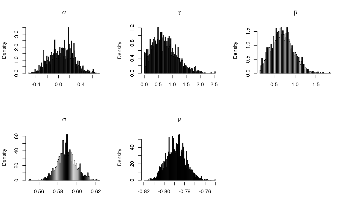
# \donttest{
# Posterior inference for Heston's model
hmod <- sde.examples("hest") # load pre-compiled model

# Simulate data
X0 <- c(X = log(1000), Z = 0.1)
theta <- c(alpha = 0.1, gamma = 1, beta = 0.8, sigma = 0.6, rho = -0.8)
dT <- 1/252
nobs <- 1000
hest.sim <- sde.sim(model = hmod, x0 = X0, theta = theta,
                    dt = dT, dt.sim = dT/10, nobs = nobs)
#> Number of normal draws required: 10000
#> Running simulation...
#> Execution time: 0 seconds.
#> Bad Draws = 0

# initialize MCMC sampler
# both components observed, no missing data between observations
init <- sde.init(model = hmod, x = hest.sim$data,
                 dt = hest.sim$dt, theta = theta)

# Initialize posterior sampling argument
nsamples <- 1e4
burn <- 1e3
hyper <- NULL # flat prior
hest.post <- sde.post(model = hmod, init = init, hyper = hyper,
                      nsamples = nsamples, burn = burn)
#> Output size:
#> params = 50000
#> Running posterior sampler...
#> Execution time: 1.41 seconds.
#> alpha accept: 44.8%
#> gamma accept: 43.7%
#> beta accept: 43.7%
#> sigma accept: 44.9%
#> rho accept: 43.7%

# plot the histogram for the sampled parameters
par(mfrow = c(2,3))
for(ii in 1:length(hmod$param.names)) {
  hist(hest.post$params[,ii],breaks=100, freq = FALSE,
       main = parse(text = hmod$param.names[ii]), xlab = "")
}
# }