Local likelihood estimation. — CondiCopLocFit • LocalCop

Estimate the bivariate copula dependence parameter eta at multiple covariate values.

CondiCopLocFit(
  u1,
  u2,
  family,
  x,
  x0,
  nx = 100,
  degree = 1,
  eta,
  nu,
  kernel = KernEpa,
  band,
  optim_fun,
  cl = NA
)

Arguments

u1: Vector of first uniform response.
u2: Vector of second uniform response.
family: An integer defining the bivariate copula family to use. See ConvertPar().
x: Vector of observed covariate values.
x0: Vector of covariate values within range(x) at which to fit the local likelihood. Does not have to be a subset of x.
nx: If x0 is missing, defaults to nx equally spaced values in range(x).
degree: Integer specifying the polynomial order of the local likelihood function. Currently only 0 and 1 are supported.
eta: Optional initial value of the copula dependence parameter (scalar). If missing will be estimated unconditionally by VineCopula::BiCopEst().
nu: Optional initial value of second copula parameter, if it exists. If missing and required, will be estimated unconditionally by VineCopula::BiCopEst(). If provided and required, will not be estimated.
kernel: Kernel function to use. Should accept a numeric vector parameter and return a non-negative numeric vector of the same length. See KernFun().
band: Kernal bandwidth parameter (positive scalar). See KernWeight().
optim_fun: Optional specification of local likelihood optimization algorithm. See Details.
cl: Optional parallel cluster created with parallel::makeCluster(), in which case optimization for each element of x0 will be done in parallel on separate cores. If cl == NA, computations are run serially.

Value

List with the following elements:

x: The vector of covariate values x0 at which the local likelihood is fit.
eta: The vector of estimated dependence parameters of the same length as x0.
nu: The scalar value of the estimated (or provided) second copula parameter.

Details

By default, optimization is performed with the quasi-Newton algorithm provided by stats::nlminb(), which uses gradient information provided by automatic differentiation (AD) as implemented by TMB.

If the default method is to be overridden, optim_fun should be provided as a function taking a single argument corresponding to the output of CondiCopLocFun(), and return a scalar value corresponding to the estimate of eta at a given covariate value in x0. Note that TMB calculates the negative local (log)likelihood, such that the objective function is to be minimized. See Examples.

Examples

# simulate data
family <- 5 # Frank copula
n <- 1000
x <- runif(n) # covariate values
eta_fun <- function(x) 2*cos(12*pi*x) # copula dependence parameter
eta_true <- eta_fun(x)
par_true <- BiCopEta2Par(family, eta = eta_true)
udata <- VineCopula::BiCopSim(n, family=family,
                              par = par_true$par)

# local likelihood estimation
x0 <- seq(min(x), max(x), len = 100)
band <- .02
system.time({
  eta_hat <- CondiCopLocFit(u1 = udata[,1], u2 = udata[,2],
                            family = family, x = x, x0 = x0, band = band)
})
#>    user  system elapsed 
#>   0.194   0.008   0.201 

# custom optimization routine using stats::optim (gradient-free)
my_optim <- function(obj) {
  opt <- stats::optim(par = obj$par, fn = obj$fn, method = "Nelder-Mead")
  return(opt$par[1]) # always return constant term, even if degree > 0
}
system.time({
  eta_hat2 <- CondiCopLocFit(u1 = udata[,1], u2 = udata[,2],
                             family = family, x = x, x0 = x0, band = band,
                             optim_fun = my_optim)
})
#>    user  system elapsed 
#>   0.373   0.004   0.378 

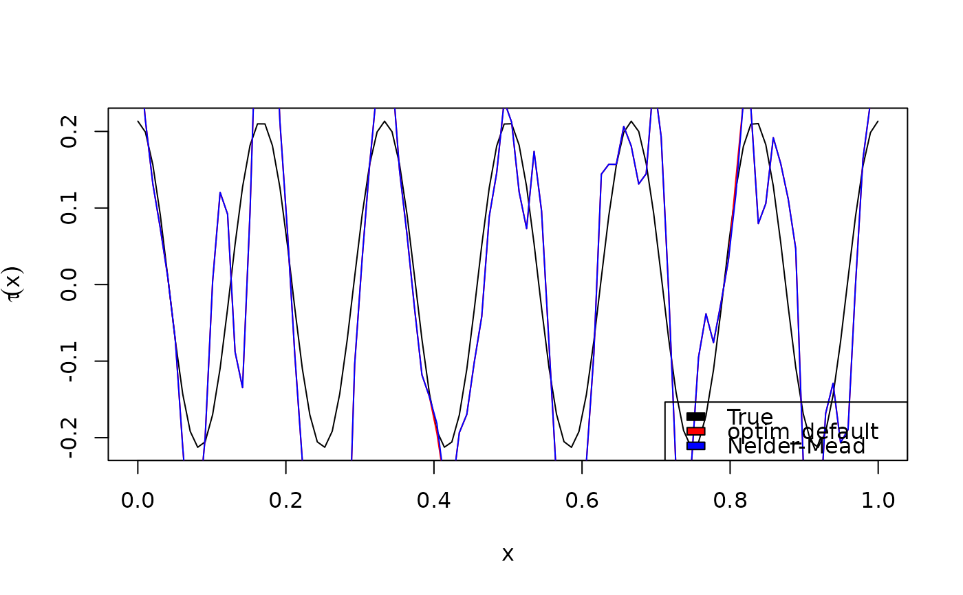
plot(x0, BiCopEta2Tau(family, eta = eta_fun(x0)), type = "l",
     xlab = expression(x), ylab = expression(tau(x)))
lines(x0, BiCopEta2Tau(family, eta = eta_hat$eta), col = "red")
lines(x0, BiCopEta2Tau(family, eta = eta_hat2$eta), col = "blue")
legend("bottomright", fill = c("black", "red", "blue"),
       legend = c("True", "optim_default", "Nelder-Mead"))