LocalCop: Local likelihood inference for conditional copulas
Elif F. Acar, Martin Lysy
2024-03-17
Source:vignettes/LocalCop.Rmd
LocalCop.RmdOverview
This vignette shows how to use the LocalCop package to conduct local likelihood inference for the dependence parameters in conditional copula models, based on the works Acar, Craiu, and Yao (2011), Acar, Craiu, and Yao (2013) and Acar, Czado, and Lysy (2019).
LocalCop is primarily intended for users who want to apply conditional copula models to real-world data with an interest to infer covariate effects on the conditional dependence between two response variables. This is done semiparametrically using kernel smoothing within the likelihood framework as detailed below.
Data generating model
For any bivariate response vector \((Y_1, Y_2)\), the conditional joint distribution given a covariate \(X\) is given by \[\begin{equation} F_X(y_1, y_2 \mid x) = C_X (F_{1\mid X} (y_1 \mid x),F_{2\mid X} (y_2 \mid x) \mid x ), \tag{1} \end{equation}\] where \(F_{1\mid X}(y_1 \mid x)\) and \(F_{2\mid X}(y_2 \mid x)\) are the conditional marginal distributions of \(Y_1\) and \(Y_2\) given \(X\), and \(C_X(u, v \mid x)\) is a conditional copula function. That is, for given \(X = x\), the function \(C_X(u, v \mid x)\) is a bivariate CDF with uniform margins.
If the true conditional marginal distrutions are known, we may compute the marginally uniform variables \(U = F_{1|X}(Y_1 \mid X)\) and \(V = F_{2|X}(Y_2 \mid X)\). In practice these distributions are unknown, such that \(\hat U = \hat F_{1|X}(Y_1 \mid X)\) and \(\hat V = \hat F_{1|X}(Y_2 \mid X)\) are pseudo-uniform variables estimated using parametric or nonparametric techniques – see Acar, Czado, and Lysy (2019) for an application using ARMA-GARCH models. Either way, the focus of LocalCop is on estimating the conditional copula function, which is given the semi-parametric model \[\begin{equation} C_X(u, v \mid x) = \mathcal{C}(u, v; \theta(x), \nu), \tag{2} \end{equation}\] where \(\mathcal{C}(u, v \; \theta, \nu)\) is one of the parametric copula families listed in Table 1, the copula dependence parameter \(\theta \in \Theta\) is an arbitrary function of \(X\), and \(\nu \in \Upsilon\) is an additional copula parameter present in some models. Since most parametric copula families have a restricted range \(\Theta \subsetneq \mathbb{R}\), we describe the data generating model (DGM) in terms of the calibration function \(\eta(x)\), such that \[\begin{equation} \theta(x) = g^{-1}(\eta(x)), \end{equation}\] where \(g^{-1}: \mathbb{R} \to \Theta\) an inverse-link function which ensures that the copula parameter has the correct range. The choice of \(g^{-1}(\eta)\) is not unique and depends on the copula family. Table 1 displays the copula function \(\mathcal{C}(u, v \mid \theta, \nu)\) for each of the copula families provided by LocalCop, along with other relevant information including the canonical choice of the inverse link function \(g^{-1}(\eta)\). In Table 1, \(\Phi^{-1}(p)\) denotes the inverse CDF of the standard normal; \(t_{\nu}^{-1}(p)\) denotes the inverse CDF of the Student-t with \(\nu\) degrees of freedom; \(\Phi_{\theta}(z_1, z_2)\) denotes the CDF of a bivariate normal with mean \((0, 0)\) and variance \(\left[\begin{smallmatrix}1 & \theta \\ \theta & 1\end{smallmatrix}\right]\); and \(t_{\theta,\nu}(z_1, z_2)\) denotes the CDF of a bivariate Student-t with location \((0, 0)\), scale \(\left[\begin{smallmatrix}1 & \theta \\ \theta & 1\end{smallmatrix}\right]\), and degrees of freedom \(\nu\).
| Family | \(\mathcal{C}(u, v \mid \theta,\nu)\) | \(\theta \in \Theta\) | \(\nu \in \Upsilon\) | \(g^{-1}(\eta)\) | \(\tau(\theta)\) |
|---|---|---|---|---|---|
| Gaussian | \(\Phi_\theta ( \Phi^{-1}(u), \Phi^{-1}(v))\) | \((-1,1)\) |
|
\(\dfrac{e^{\eta} - e^{-\eta}}{e^{\eta} + e^{-\eta}}\) | \(\frac{2}{\pi}\arcsin(\theta)\) |
| Student-t | \(t_{\theta,\nu} ( t_\nu^{-1}(u), t_\nu^{-1}(v))\) | \((-1,1)\) | \((0, \infty)\) | \(\dfrac{e^{\eta} - e^{-\eta}}{e^{\eta} + e^{-\eta}}\) | \(\frac{2}{\pi}\arcsin(\theta)\) |
| Clayton | \(\displaystyle (u^{-\theta} + v^{-\theta} -1)^{-\frac{1}{\theta}}\) | \((0, \infty)\) |
|
\(e^\eta\) | \(\frac{\theta}{\theta + 2}\) |
| Gumbel | \(\displaystyle \exp\left[ - \{ (-\log u)^\theta + (-\log v)^\theta\}^{\frac{1}{\theta}} \right]\) | \([1, \infty)\) |
|
\(e^\eta + 1\) | \(1 - \frac{1}{\theta}\) |
| Frank | \(-\frac{1}{\theta}\log \left\{ 1 + \frac{(e^{-\theta u} - 1)(e^{-\theta v} - 1)}{e^{-\theta} - 1}\right\}\) | \((-\infty, \infty)\setminus\{0\}\) |
|
\(\eta\) | no closed form |
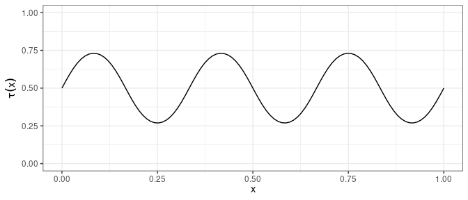
The code below shows how to simulate data from model (2) using the Gumbel family, where the change in Kendall \(\tau\) as a function of the covariate in displayed in Figure 1.
# simulate copula data given a covariate
set.seed(2024)
family <- 4  # Gumbel Copula
n <- 1000    # number of observations
x <- sort(runif(n))  # covariate values
eta_fun <- function(x) sin(6*pi*x) # calibration function

# simulate data
eta_true <- eta_fun(x)
par_true <- BiCopEta2Par(family = family, eta = eta_true) # copula parameter
udata <- VineCopula::BiCopSim(n, family = family, par = par_true$par)

# plot tau(x)
tibble(
  x = seq(0, 1, len = 100),
) %>%
  mutate(
    tau = BiCopEta2Tau(family, eta = eta_fun(x))
  ) %>%
  ggplot(aes(x = x, y = tau)) +
  geom_line() +
  ylim(c(0, 1)) +
  xlab(expression(x)) + ylab(expression(tau(x))) +
  theme_bw()
Figure 1: Conditional Kendall \(\tau\) for Gumbel copula under DGM.
Local likelihood estimation of the dependence parameter
Local likelihood estimation uses Taylor expansions to approximate the dependence parameter function at an observed covariate value \(X = x\) near a fixed point \(X = x_0\), i.e.,
\[
\eta(x)\approx \eta(x_0) + \eta^{(1)}(x_0) (x - x_0) + \ldots + \dfrac{\eta^{(p)}(x_0)}{p!} (x - x_0)^{p}.
\]
One then estimates \(\beta_k = \eta^{(k)}(x_0)/k!\) for \(k = 0,\ldots,p\) using a kernel-weighted local likelihood function
\[\begin{equation}
\ell(\boldsymbol{\beta}) = \sum_{i=1}^n \log\left\{ c\left(u_i, v_i ; g^{-1}( \boldsymbol{x}_{i}^T \boldsymbol{\beta}), \nu \right)\right\} K_h\left(\dfrac{x_i-x_0}{h}\right),
\tag{3}
\end{equation}\]
where \((u_i, v_i, x_i)\) is the data for observation \(i\), \(\boldsymbol{x}_i = (1, x_i - x_0, (x_i - x_0)^2, \ldots, (x_i - x_0)^p)\), \(\boldsymbol{\beta}= (\beta_0, \beta_1, \ldots, \beta_p)\), and \(K_h(z)\) is a kernel function with bandwidth parameter \(h > 0\). Having maximized \(\ell(\boldsymbol{\beta})\) in (3), one estimates \(\eta(x_0)\) by \(\hat \eta(x_0) = \hat \beta_0\). Usually, a linear fit with \(p=1\) suffices to obtain a good estimate in practice. The estimation procedure for a single value of \(X = x_0\) for given copula family and bandwidth parameter is carried out by CondiCopLocFit().
x0 <- 0.1
band <- 0.1
degree <- 1
kernel <- KernEpa # Epanichov kernel (default value)
fit1 <- CondiCopLocFit(
  u1 = udata[,1], u2 = udata[,2], x = x,
  x0 = x0,
  family = family,
  degree = degree,
  kernel = kernel,
  band = band
)
fit1
#> $x
#> [1] 0.1
#>
#> $eta
#> [1] 0.839931
#>
#> $nu
#> [1] 0
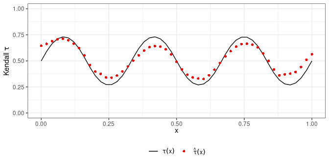
Repeating this procedure over a grid of covariate values produces an estimate \(\hat \eta(x)\) of the underlying dependence function. This can also be accomplished with CondiCopLocFit() as shown below.
x0 <- seq(0, 1, by=0.02)
fitseq <- CondiCopLocFit(
  u1 = udata[,1], u2 = udata[,2], x = x,
  x0 = x0,
  family = family,
  degree = degree,
  kernel = kernel,
  band = band
)

# plot true vs fitted tau
legend_names <- c(expression(tau(x)),
                  expression(hat(tau)(x)))
tibble(
  x = x0,
  True = BiCopEta2Tau(family, eta = eta_fun(x0)),
  Fitted = BiCopEta2Tau(fitseq$eta, family= family)
) %>%
  pivot_longer(True:Fitted,
               names_to = "Type", values_to = "y") %>%
  mutate(
    Type = factor(Type, levels = c("True", "Fitted"))
  ) %>%
  ggplot(aes(x = x, y = y, group = Type)) +
  geom_line(aes(color = Type, linetype = Type)) +
  geom_point(aes(shape = Type, color = Type)) +
  scale_color_manual(values = c("black", "red"), labels = legend_names) +
  scale_shape_manual(values = c(NA, 16), labels = legend_names) +
  scale_linetype_manual(values = c("solid", NA), labels = legend_names) +
  ylim(c(0, 1)) +
  xlab(expression(x)) + ylab(expression("Kendall "*tau)) +
  theme_bw() +
  theme(
    legend.position = "bottom",
    legend.title = element_blank()
  )
Figure 2: Conditional Kendall \(\tau\) estimates under the Gumbel copula using bandwidth \(h=0.1\).
Copula Selection and Model Tuning
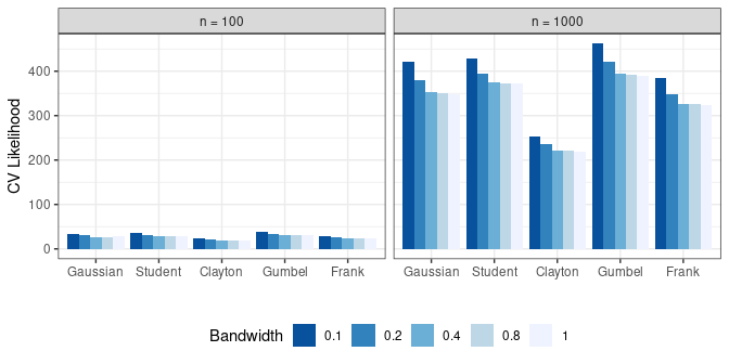
Selection of the copula family and bandwidth parameter is done via leave-one-out cross-validation (LOO-CV) as described in Acar, Czado, and Lysy (2019). To reduce the computation time in model selection, we may calculate the LOO-CV for just a subset of the sample.
bandset <- c(0.1, 0.2, 0.4, 0.8, 1) # bandwidth set
famset <- c(1, 2, 3, 4, 5) # family set
n_loo <- 100  # number of leave-one-out observations in CV likelihood calculation
system.time({
  cvselect1 <- CondiCopSelect(
    u1 = udata[,1], u2 = udata[,2], x = x,
    family = famset,
    degree = degree,
    kernel = kernel,
    band = bandset,
    xind = n_loo
  )
})
cv_res1 <- cvselect1$cv
cv_res1
#>    band family       cv
#> 1   0.1      1 33.72408
#> 2   0.2      1 30.22907
#> 3   0.4      1 26.91116
#> 4   0.8      1 27.22770
#> 5   1.0      1 27.54328
#> 6   0.1      2 34.95500
#> 7   0.2      2 31.06883
#> 8   0.4      2 28.20758
#> 9   0.8      2 28.92498
#> 10  1.0      2 29.21409
#> 11  0.1      3 23.26226
#> 12  0.2      3 20.51586
#> 13  0.4      3 17.96064
#> 14  0.8      3 18.34648
#> 15  1.0      3 18.45101
#> 16  0.1      4 38.68924
#> 17  0.2      4 34.64196
#> 18  0.4      4 30.75936
#> 19  0.8      4 31.43345
#> 20  1.0      4 31.77389
#> 21  0.1      5 29.72769
#> 22  0.2      5 25.59749
#> 23  0.4      5 23.23388
#> 24  0.8      5 24.02684
#> 25  1.0      5 24.43723
The leave-one-out cross-validation for the full sample is provided below for comparisons.
system.time({
  cvselect2 <- CondiCopSelect(
    u1 = udata[,1], u2 = udata[,2], x = x,
    family = famset,
    degree = degree,
    kernel = kernel,
    band = bandset,
    xind = nrow(udata)
  )
})
cv_res2 <- cvselect2$cv
cv_res2
#>    band family       cv
#> 1   0.1      1 422.2925
#> 2   0.2      1 380.4366
#> 3   0.4      1 353.6886
#> 4   0.8      1 350.2815
#> 5   1.0      1 348.7304
#> 6   0.1      2 428.2676
#> 7   0.2      2 395.4231
#> 8   0.4      2 374.7095
#> 9   0.8      2 373.3327
#> 10  1.0      2 372.6614
#> 11  0.1      3 252.9172
#> 12  0.2      3 234.8385
#> 13  0.4      3 221.4233
#> 14  0.8      3 220.4843
#> 15  1.0      3 219.8683
#> 16  0.1      4 461.6522
#> 17  0.2      4 421.7474
#> 18  0.4      4 394.1287
#> 19  0.8      4 391.4590
#> 20  1.0      4 390.0860
#> 21  0.1      5 384.3447
#> 22  0.2      5 347.7702
#> 23  0.4      5 325.6584
#> 24  0.8      5 325.0720
#> 25  1.0      5 324.6259
Figure 3 displays the LOO-CV metric (larger is better) for both the full sample (\(n = 1000\)) and a subset of the sample (\(n = 100\)). The rank of each combination of family and bandwidth is very similar in both settings. In particular, i both cases we select the Gumbel copula with bandwidth parameter \(h = 0.1\). This suggests that subset-based model selection can be used to reduce the computation time.
fam_names <- c("Gaussian", "Student", "Clayton", "Gumbel", "Frank")
bind_rows(as_tibble(cvselect1$cv) %>%
          mutate(n = n_loo),
          as_tibble(cvselect2$cv) %>%
          mutate(n = nrow(udata))) %>%
  mutate(
    family = factor(family, levels = c(1,2,3,4,5),
                    labels = fam_names),
    Bandwidth = factor(band),
    n = factor(paste0("n = ", n))
  ) %>%
  ggplot(aes(x = family, y  = cv, fill = Bandwidth)) +
  geom_bar(stat="identity", position = "dodge") +
  facet_grid(. ~ n) +
  scale_fill_brewer(palette="Blues", direction=-1) +
  xlab("") + ylab("CV Likelihood") +
  theme_bw() +
  theme(legend.position = "bottom",
        legend.direction = "horizontal")
Figure 3: Cross-validated likelihood for copula and bandwidth selection based on a subset and the full sample.
Sensitivity to the choice of copula family
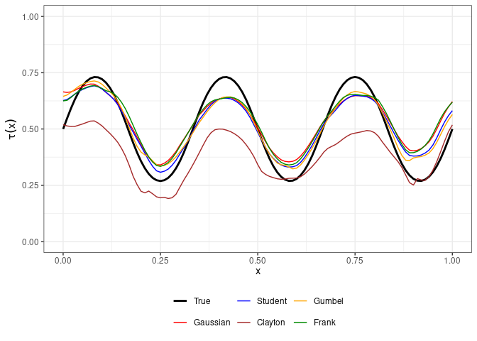
Figure 4 displays the true and estimated conditional Kendall \(\tau\) for each of the copula families using the selected bandwidth parameter \(h = 0.1\). The results suggest that misspecification of the copula family does not drastically affect the local likelihood estimates of \(\tau(x)\), except for the Clayton copula which shows the most departure from the Gumbel copula used in the DGM.
x0 <- seq(0, 1, by=0.01)
tau_est <- sapply(1:5, function(fam_id) {
  fit <- CondiCopLocFit(
    u1 = udata[,1], u2 = udata[,2], x = x,
    x0 = x0,
    family = fam_id,
    degree = degree,
    kernel = kernel,
    band = band)
  BiCopEta2Tau(fit$eta, family=fam_id)
})

colnames(tau_est) <- fam_names

as_tibble(tau_est) %>%
  mutate(
    x = x0,
    True = BiCopEta2Tau(family, eta = eta_fun(x0))
  ) %>%
  pivot_longer(!x, names_to = "Type", values_to = "tau") %>%
  mutate(
    Type = factor(Type, levels = c("True", fam_names))
  ) %>%
  ggplot(aes(x = x, y = tau, group = Type)) +
  geom_line(aes(col = Type, linewidth = Type)) +
  scale_color_manual(
    values = c("black", "red", "blue", "brown", "orange", "green4")
  ) +
  scale_linewidth_manual(values = c(1, rep(.5, 5))) +
  ylim(c(0, 1)) +
  xlab(expression(x)) + ylab(expression(tau(x))) +
  theme_bw() +
  theme(
    legend.position = "bottom",
    legend.title = element_blank(),
  )
Figure 4: Conditional Kendall \(\tau\) estimates under different copula families.