Fast Inference for Common-Factor Stochastic Volatility Models
Martin Lysy
University of Waterloo
University of Waterloo
2024-09-10
Source:vignettes/svcommon.Rmd
svcommon.RmdThe Common-Factor Multivariate Stochastic Volatility Model
Let \(X_{it}\) denote the log price of asset \(i = 1,\ldots N_a\) at time \(t\) and \(V_{it}\) denote the corresponding volatility on the standard deviation scale. The common-factor multivariate stochastic volatility (mSV) model proposed by Fang et al. (2020) is marginally written as \[\begin{equation} \begin{aligned} \mathop{}\!\mathrm{d}\log V_{it} & = -\gamma_i (\log V_{it} - \mu_i) \mathop{}\!\mathrm{d}t + \sigma_i \mathop{}\!\mathrm{d}B_{it}^V \\ \mathop{}\!\mathrm{d}X_{it} & = (\alpha_i - \tfrac 1 2 V_{it}^2) \mathop{}\!\mathrm{d}t + V_{it} \left(\rho_i \mathop{}\!\mathrm{d}B_{it}^V + \sqrt{1 - \rho_i^2} \mathop{}\!\mathrm{d}B_{it}^Z\right). \end{aligned} \tag{1} \end{equation}\] The correlation between assets and volatilities comes from factor models for both the assets and the volatilities, namely \[\begin{equation} \begin{aligned} \mathop{}\!\mathrm{d}B_{it}^V & = \tau_i \mathop{}\!\mathrm{d}B_{\star t}^V + \sqrt{1 - \tau_i^2} \mathop{}\!\mathrm{d}B_{it}^\epsilon \\ \mathop{}\!\mathrm{d}B_{it}^Z & = \omega_i \mathop{}\!\mathrm{d}B_{\star t}^Z + \sqrt{1 - \omega_i^2} \mathop{}\!\mathrm{d}B_{it}^\eta. \end{aligned} \tag{2} \end{equation}\] In Fang et al. (2020) it is suggested to estimate the volatility common innovation factor \(B_{\star t}^{V}\) via an observable proxy, for example the VIX. That is, if \(V_{\star t}\) is an observable proxy for the common volatility factor, then we use it to estimate \(B_{\star t}^V\) via \[\begin{equation} \mathop{}\!\mathrm{d}\log V_{\star t} = -\gamma_{\star} (\log V_{\star t} - \mu_{\star}) \mathop{}\!\mathrm{d}t + \sigma_{\star} \mathop{}\!\mathrm{d}B_{\star t}^V. \tag{3} \end{equation}\] Here we propose to do something similar for the asset common innovation factor \(B_{\star t}^Z\). That is, let \((X_{0t}, V_{0t})\) be a univariate stochastic volatility model for an observable proxy for the common asset factor (for example, SPX). Then we give it a similar marginal model to the above: \[\begin{equation} \begin{aligned} \mathop{}\!\mathrm{d}\log V_{0t} & = -\gamma_0 (\log V_{0t} - \mu_0) \mathop{}\!\mathrm{d}t + \sigma_0 \mathop{}\!\mathrm{d}B_{0t}^V \\ \mathop{}\!\mathrm{d}X_{0t} & = (\alpha_0 - \tfrac 1 2 V_{0t}^2) \mathop{}\!\mathrm{d}t + V_{0t} \left(\rho_0 \mathop{}\!\mathrm{d}B_{0 t}^V + \sqrt{1 - \rho_0^2} \mathop{}\!\mathrm{d}B_{0t}^Z \right), \end{aligned} \tag{4} \end{equation}\] where \(\mathop{}\!\mathrm{d}B_{0t}^V = \tau_0 \mathop{}\!\mathrm{d}B_{\star t}^V + \sqrt{1 - \tau_0^2} \mathop{}\!\mathrm{d}B_{0t}^\epsilon\). The asset common factor is estimated from the proxy by equating \(B_{\star t}^Z = B_{0t}^Z\).
Parameter Estimation
The common-factor stochastic volatility model defined by (1) through (4) has likelihood function \[ \mathcal{L}({\boldsymbol{\theta}}\mid {\boldsymbol{X}}, {\boldsymbol{V}}_0) \propto \int p({\boldsymbol{X}}, {\boldsymbol{V}}, {\boldsymbol{V}}_0 \mid {\boldsymbol{\theta}}) \mathop{}\!\mathrm{d}{\boldsymbol{V}}. \] While the integral over the latent volatilities \({\boldsymbol{V}}\) is typically intractable, svcommon uses Laplace’s method to approximate the integral by solving a tractable optimization problem. This is implemented using the R package TMB, which efficiently computes the approximate marginal loglikelihood \[\begin{equation} \ell_{\text{Lap}}({\boldsymbol{\theta}}\mid {\boldsymbol{X}}, {\boldsymbol{V}}_0) \approx \log \mathcal{L}({\boldsymbol{\theta}}\mid {\boldsymbol{X}}, {\boldsymbol{V}}_0) \tag{5} \end{equation}\] and its gradient \(\frac{\partial}{\partial {\boldsymbol{\theta}}} \ell_{\text{Lap}}({\boldsymbol{\theta}}\mid {\boldsymbol{X}}, {\boldsymbol{V}}_0)\) using automatic differentiation. svcommon uses a block coordinate descent algorithm with good initial values to very quickly converge to the approximate MLE \(\hat {\boldsymbol{\theta}}= \operatorname{arg\,max}_{{\boldsymbol{\theta}}} \ell_{\text{Lap}}({\boldsymbol{X}}, {\boldsymbol{V}}_0 \mid {\boldsymbol{\theta}})\), about two orders of magnitude faster than exact inference methods. The procedure is illustrated with a dataset consisting of 3408 daily closing prices of 46 constituents of the S&P500, the index value itself (GSPC), and its volatility index (VIX).
# required packages
library(svcommon)
library(mvtnorm) # multivariate normal draws
library(tidyr); library(dplyr) # data frame manipulation
library(ggplot2) # plotting

dim(snp500) # automatically loaded with svcommon
#> [1] 3408   48
snp500[1:6, ncol(snp500)-8 + 1:8]
#>        MRK      PFE      ABT      UNH      CVS      BMY    GSPC   VIX
#> 1 26.72457 18.33346 10.54715 28.65658 16.81109 13.58980 1091.23 16.96
#> 2 27.11290 18.48489 10.62487 28.95242 16.89979 13.76582 1098.35 16.00
#> 3 27.19528 18.43247 10.59119 28.68308 16.84911 13.67195 1095.68 15.88
#> 4 27.27176 18.36258 10.62228 28.69191 17.07720 13.64260 1096.19 15.33
#> 5 27.07761 18.58389 10.73887 28.77579 17.15745 13.94773 1104.96 14.98
#> 6 26.50687 18.81684 10.67928 28.83320 17.19124 13.94773 1105.09 14.91
Initialization
Initial guesses for the parameters of the common-factor stochastic volatility (SVC) model are obtained from marginal fits of the exponential Ornstein-Uhlenbeck (EOU) model to each asset and to GSPC. To perform the optimization, the R built-in stats package provides the optimiziers stats::optim(), stats::nlm(), and stats::nlminb(). Various experiments with SVC modeling indicate that statss:nlminb() is by far the fastest, with little difference in numerical accuracy. Indeed, the marginal fits are extremely fast and stable, even with the (log or logit) parameters arbitrarily initialized to zero.
# problem dimensions
nobs <- 1000 # number of days
nasset <- 5 # number of assets, excluding GSPC

# format the data
dt <- 1/252
Xt <- as.matrix(cbind(GSPC = snp500[1:nobs, "GSPC"],
                      snp500[1:nobs, 1+1:nasset]))
Xt <- log(Xt)
log_VPt <- log(as.numeric(snp500[1:nobs, "VIX"]))

# initialize latent variables with rolling window standard deviations
log_Vt <- log(apply(Xt, 2, sv_init, dt = dt, block_size = 10))
# initialize parameters with default values
alpha <- rep(0, nasset+1)
log_gamma <- rep(0, nasset+2)
mu <- rep(0, nasset+2)
log_sigma <- rep(0, nasset+2)
logit_rho <- rep(0, nasset+1)
logit_tau <- rep(0, nasset+1)
logit_omega <- rep(0, nasset)

# parameter and latent variable list for convenient updating
curr_par <- list(log_Vt = log_Vt,
                 alpha = alpha,
                 log_gamma = log_gamma,
                 mu = mu,
                 log_sigma = log_sigma,
                 logit_rho = logit_rho,
                 logit_tau = logit_tau,
                 logit_omega = logit_omega)

# optimization control parameters
opt_control <- list(eval.max = 1000, iter.max = 1000, trace = 10)

# initialize parameters of each individual asset
tm_tot <- system.time({
  for(iasset in 0:nasset) {
    message("asset = ", iasset)
    # construct model object
    eou_ad <- eou_MakeADFun(Xt = Xt[,iasset+1], dt = dt,
                            alpha = curr_par$alpha[iasset+1],
                            log_Vt = curr_par$log_Vt[,iasset+1],
                            log_gamma = curr_par$log_gamma[iasset+2],
                            mu = curr_par$mu[iasset+2],
                            log_sigma = curr_par$log_sigma[iasset+2],
                            logit_rho = curr_par$logit_rho[iasset+1])
    # optimize with quasi-newton method
    tm <- system.time({
      opt <- nlminb(start = eou_ad$par,
                    objective = eou_ad$fn,
                    gradient = eou_ad$gr,
                    control = opt_control)
    })
    message("Time: ", round(tm[3], 2), " seconds")
    # update parameters
    curr_par <- svc_update(eou_ad, old_par = curr_par, iasset = iasset)
  }
})
message("Total Time: ", round(tm_tot[3], 2), " seconds.")
Blockwise Coordinate Descent
The following algorithm updates the parameters for each asset conditioned on the values of all the others. Note that the Laplace approximation in this case depends only on the latent volatilities of the given asset and that of the asset common factor. Thus, svcommon removes the other volatilities from the gradient calculations, which considerably speeds up the calculations.
Here, nepoch denotes the number of cycles through all assets. For this dataset it appears that after nepoch = 3 the parameter values are changing very little.
nepoch <- 3

tm_tot <- system.time({
  for(iepoch in 1:nepoch) {
    message("epoch = ", iepoch)
    for(iasset in -1:nasset) {
      message("asset = ", iasset)
      svc_ad <- svc_MakeADFun(Xt = Xt, log_VPt = log_VPt, dt = dt,
                              par_list = curr_par,
                              iasset = iasset)
      tm <- system.time({
        opt <- nlminb(start = svc_ad$par,
                      objective = svc_ad$fn,
                      gradient = svc_ad$gr,
                      control = opt_control)
      })
      message("Time: ", round(tm[3], 2), " seconds")
      curr_par <- svc_update(svc_ad, old_par = curr_par, iasset = iasset)
    }
  }
})
message("Total Time: ", round(tm_tot[3], 2), " seconds.")
For good measure, let’s finish with a joint optimization over all parameters. This should be comparatively fast now that the optimizer has good starting values1.
# joint parameter optimization
iasset <- "all"
svc_ad <- svc_MakeADFun(Xt = Xt, log_VPt = log_VPt, dt = dt,
                        par_list = curr_par,
                        iasset = iasset)
tm <- system.time({
  opt <- nlminb(start = svc_ad$par,
                objective = svc_ad$fn,
                gradient = svc_ad$gr,
                control = opt_control)
})
message("Time: ", round(tm[3], 2), " seconds")
curr_par <- svc_update(svc_ad, old_par = curr_par, iasset = iasset)
Bayesian Estimation and Forecasting
Let’s take a look at the parameter estimates.
system.time({
  svc_est <- TMB::sdreport(svc_ad)
})| Estimate | Std. Error | |
|---|---|---|
| alpha | 0.05 | 0.05 |
| alpha | 0.01 | 0.07 |
| alpha | 0.02 | 0.08 |
| alpha | -0.05 | 0.07 |
| alpha | -0.01 | 0.07 |
| alpha | 0.00 | 0.06 |
| log_gamma | 1.78 | 0.13 |
| log_gamma | 1.13 | 0.21 |
| log_gamma | 1.54 | 0.25 |
| log_gamma | 1.67 | 0.28 |
| log_gamma | 1.66 | 0.25 |
| log_gamma | 1.79 | 0.23 |
| log_gamma | 1.44 | 0.33 |
| mu | 2.69 | 0.08 |
| mu | -2.12 | 0.10 |
| mu | -1.74 | 0.15 |
| mu | -1.65 | 0.13 |
| mu | -1.66 | 0.19 |
| mu | -1.72 | 0.12 |
| mu | -1.84 | 0.16 |
| log_sigma | 0.00 | 0.02 |
| log_sigma | -0.39 | 0.09 |
| log_sigma | 0.42 | 0.11 |
| log_sigma | 0.37 | 0.13 |
| log_sigma | 0.75 | 0.10 |
| log_sigma | 0.44 | 0.13 |
| log_sigma | 0.38 | 0.12 |
| logit_rho | -3.10 | 0.09 |
| logit_rho | -1.35 | 0.09 |
| logit_rho | -1.47 | 0.09 |
| logit_rho | -1.53 | 0.10 |
| logit_rho | -1.57 | 0.10 |
| logit_rho | -1.61 | 0.11 |
| logit_tau | 2.93 | 0.08 |
| logit_tau | 2.92 | 0.26 |
| logit_tau | 2.96 | 0.26 |
| logit_tau | 1.93 | 0.14 |
| logit_tau | 2.32 | 0.16 |
| logit_tau | 2.34 | 0.17 |
| logit_omega | 2.22 | 0.11 |
| logit_omega | 2.26 | 0.12 |
| logit_omega | 1.48 | 0.10 |
| logit_omega | 2.16 | 0.13 |
| logit_omega | 2.07 | 0.13 |
| log_VT | -1.65 | 0.05 |
| log_VT | -0.81 | 0.13 |
| log_VT | -0.90 | 0.13 |
| log_VT | 0.12 | 0.13 |
| log_VT | -0.74 | 0.12 |
| log_VT | -0.95 | 0.14 |
All parameter estimates have reasonable precision, except notably \(\alpha_i\), the long-term trend in asset \(i\), which is notoriously difficult to estimate. Also included are stimates of \(\log V_{iT}\), the latent volatility on the last day \(t = T\) in the observed data. This can be useful for Bayesian forecasting, which can be conducted using the following method:
Let \(p({\boldsymbol{\theta}}, \log V_{0T}, \ldots, \log V_{qT} \mid {\boldsymbol{X}}, {\boldsymbol{V}}_0)\) denote the posterior distribution of the parameters and terminal volatilities for \(q\) assets and the common asset factor with the Lebesgue prior2 \(\pi({\boldsymbol{\theta}}) \propto 1\). By the mode-quadrature approximation, this posterior is taken to be normal with mean and variance obtained from
TMB::sdreport().Let \(p(X_{0,T+d}, \ldots, X_{q,T+d}, \log V_{0,T+d}, \ldots, \log V_{q,T+d} \mid {\boldsymbol{X}}, {\boldsymbol{V}}_0)\) denote the Bayesian forecast distribution for assets and volatilities on day \(t = T+d\). We can simulate from this distribution by combining draws from the multivariate normal approximation to \(p({\boldsymbol{\theta}}, \log V_{0T}, \ldots, \log V_{qT} \mid {\boldsymbol{X}}, {\boldsymbol{V}}_0)\) with forward simulation from the SVC model with
svc_sim().
An illustration of this procedure produces the posterior forecast distribution in Figure 1.
nfwd <- 10 # number of days to forecast
nsim <- 1e4 # number of simulated forecasts

# sample from the mode-quadrature approximation
curr_post <- mvtnorm::rmvnorm(nsim,
                              mean = svc_est$value,
                              sigma = svc_est$cov)

# convert to appropriate inputs to svc_sim
sim_args <- sapply(c("alpha", "log_gamma", "mu", "log_sigma", "logit_rho",
                       "logit_tau", "logit_omega", "log_VT"),
                     function(nm) {
                       t(curr_post[,colnames(curr_post) == nm])
                     }, simplify = FALSE)
names(sim_args)[8] <- "log_V0" # rename log_VT
# remaining arguments
sim_args <- c(sim_args,
              list(X0 = Xt[nobs,],
                   log_VP0 = log_VPt[nobs],
                   nobs = nfwd, dt = dt))
# forward simulation
fwd_post <- do.call(svc_sim, args = sim_args)

# plot posteriors on day t = nobs + nfwd
# format data
X_fwd <- t(fwd_post$Xt[nfwd,,])
colnames(X_fwd) <- colnames(Xt)
X_fwd <- data.frame(type = "X", X_fwd)
V_fwd <- exp(t(fwd_post$log_Vt[nfwd,,]))
colnames(V_fwd) <- colnames(log_Vt)
V_fwd <- data.frame(type = "V", V_fwd)
XV_fwd <- rbind(X_fwd, V_fwd) %>%
  as_tibble()
# plot
XV_fwd %>%
  pivot_longer(GSPC:USB, names_to = "Asset", values_to = "Value") %>%
  mutate(Asset = factor(Asset, levels = colnames(Xt))) %>%
  ggplot(aes(x = Value, group = Asset)) +
  geom_density(aes(color = Asset)) +
  facet_wrap(~ type, scales = "free", ncol = 2) +
  xlab("") + ylab("Posterior Forecast Distribution")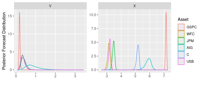
Figure 1: Posterior forecast distribution \(p({\boldsymbol{V}}_{T+d} \mid {\boldsymbol{X}}, {\boldsymbol{V}}_0)\) and \(p({\boldsymbol{X}}_{T+d} \mid {\boldsymbol{X}}, {\boldsymbol{V}}_0)\).
References
For this particular dataset, it is possible to skip the initialization and blockwise coordinate descent steps, provided the
iter.maxparameter tostats::nlminb()is large enough.↩︎Since the prior is flat on the original scale but optimization is done on the transformed scale (\(\log \gamma_i\), \(\operatorname{logit}\rho_i\), etc.) the optimizer provides the correct Bayesian mode but a penalized maximum likelihood. SVC experiments indicate that penalization considerably improves the estimation of correlation parameters, which otherwise tend to drift off to boundary values.↩︎