5 Introduction to Longitudinal Data

Author: Grace Tompkins

Last Updated: March 25, 2022

---

5.1 Introduction

Longitudinal studies are studies in which we follow and take repeated measurements from a sample of individuals over a certain period of time. The major advantage of a longitudinal study is that one can distinguish between the outcome changes within a subject over time (longitudinal effect) and the differences among subjects at a given point in time (cohort effect). Longitudinal studies can also separate time effects and quantify different sources of variation in the data by separating the between-subject and within-subject variation. Cross-sectional studies, in which we see data only at one “snapshot” or point in time, do not have these benefits.

While longitudinal studies can either be prospective (subjects are followed forward in time) or retrospective (measurements on subjects are extracted historically), prospective studies tend to be preferred. This is because in retrospective studies there exists recall bias, where subjects inaccurately remember past events, which can impact the data collected and consequently the resultant analysis and findings (Diggle et al. 2002).

A challenge of longitudinal data is that observations taken within each subject are correlated. For example, weather patterns tend to be correlated at a given location, in the sense that if today is rainy then we are more likely to have a rainy day tomorrow than a sunny day. In general, even when we have a great amount of time separation between observations, the correlation between a pair of responses on the same subject rarely approaches zero (Fitzmaurice, Laird, and Ware 2011). We refer to the correlation of responses within the same individual as the intra-subject correlation. This implies that our typical statistical modeling tools which assume independence among observations are inappropriate for this type of data. Methods that account for intra-subject correlation will be discussed further in the following sections, and include linear models, linear mixed effect (LME) models, generalized linear mixed effects models (GLMMs), and generalized estimating equations (GEEs).

While longitudinal analysis is often used in the context of health data involving repeated measurements from patients, it can also be found in a variety of disciplines, including (but not limited to) economics, finance, environmental studies, and education.

A working example of a dentistry data set with a continuous outcome will be carried through this module, with R code accompanying the theory presented. If the statistical theory presented in each section is not of interest to the reader, the working example should be able to be followed on its own. At the end of each section that presents new methodology, a second example will be fully worked through using the methods presented.

5.1.1 List of R packages Used

In this chapter, we will be using the packages geesmv, nmle, ggplot2, emdbook, lattice.

library(geesmv) # load the required packages
library(nlme)
library(ggplot2)
library(emdbook)
library(lattice)

5.1.2 Motivating Example

For the first working example, we consider the data set dental from the R package geesmv.

We can first load the data set dental to the working environment.

data("dental") # load the data dental from the geesmv package

# update name of gender variable to be sex, as described in documentation of data set
colnames(dental) <- c("subject", "sex", "age_8", "age_10", "age_12", "age_14")

This data set was obtained to study the growth of 27 children (16 boys and 11 girls), which contains an orthodontic measurement (the distance from the center of the pituitary to the pterygomaxillary fissure) in millimeters, and the sex assigned at birth for each child. Orthodontic measurements were at ages 8 (baseline), 10, 12, and 14 years for each child. To learn more about the data set and its covariates, one can type ?dental in the R Console after loading the geesmv package.

To assess the form of the data, we can look at the first six observations using the head() function:

head(dental) # look at the first 6 observations in the data set

##   subject sex age_8 age_10 age_12 age_14
## 1       1   F  21.0   20.0   21.5   23.0
## 2       2   F  21.0   21.5   24.0   25.5
## 3       3   F  20.5   24.0   24.5   26.0
## 4       4   F  23.5   24.5   25.0   26.5
## 5       5   F  21.5   23.0   22.5   23.5
## 6       6   F  20.0   21.0   21.0   22.5

In this data set, the subject variable identifies the specific child and the sex variable is a binary variable such that sex = F when the subject is female and sex = M if male. The last four columns show the orthodontic measurements for each child at the given age, which are continuous.

Using this data, we want to ask the following questions:

• Do the orthodontic measurements increase as the age of the subjects increases?
• Is there a difference in growth by sex assigned at birth?

In order to answer these, we need to employ longitudinal methods, which will be described in the following sections.

5.2 Data Structure for Longitudinal Responses

Longitudinal data can be presented or stored in two different ways. Wide form data has a single row for each subject and a unique column for the response of the subject at different time points. In its unaltered form, the dental data set is in wide form. However, we often need to convert our data into long form in order to use many popular software packages for longitudinal data analysis. In long form, we have multiple rows per subject representing the outcome measured at different time points. We also include an additional variable denoting the time or occasion in which we obtained the measurement.

As an example, let’s change the dental data set into the long form. We can do this by employing the reshape() function in R. The reshape() function has many arguments available, which can be explored by typing ?reshape in the console. Some of the important arguments, which we will be using for this example, include:

• data: the data set we are converting, as a dataframe object in R;
• direction: the direction in which we are converting to;
• idvar: the column name of the variable identifying subjects (typically some type of id, or name);
• varying: the name of the sets of variables in the wide format that we want to transform into a single variable in long format (“time-varying”). Typically these are the column names of wide form data set in which the repeated outcome is measured;
• times: the values we are going to use in the long form that indicates when the observations were taken;
• timevar: the name of the variable in long form indicating the time; and
• drop: a vector of column names that we do not want to include in the newly reshaped data set.

To reshape the wide form dental data set into long form, we can execute the following code:

# reshape the data into long form
dental_long <- reshape(
  data = dental, # original data in wide form
  direction = "long", # changing from wide TO long
  idvar = "subject", # name of variable indicating unique
  # subjects in wide form data set
  varying = c("age_8", "age_10", "age_12", "age_14"), # name
  # of variables in which outcomes recorded
  v.names = "distance", # assigning a new name to the outcome
  times = c(8, 10, 12, 14), # time points in which the above
  # outcomes were recorded
  timevar = "age"
) # name of the time variable we're using

# order the data by subject ID and then by age
dental_long <- dental_long[order(dental_long$subject, dental_long$age), ]

# look at the first 10 observations
head(dental_long, 10)

##      subject sex age distance
## 1.8        1   F   8     21.0
## 1.10       1   F  10     20.0
## 1.12       1   F  12     21.5
## 1.14       1   F  14     23.0
## 2.8        2   F   8     21.0
## 2.10       2   F  10     21.5
## 2.12       2   F  12     24.0
## 2.14       2   F  14     25.5
## 3.8        3   F   8     20.5
## 3.10       3   F  10     24.0

We see that the distance variable corresponds to the values in one of the last four columns of the dental data set in wide form for each subject. For the rest of the example, we will be using the data stored in dental_long.

5.3 Linear Models for Continuous Outcome

5.3.1 Assumptions

When we are analyzing data that has a continuous outcome, we can often use a linear model to answer our research questions. In this setting, we require that

• the data set has a balanced design, meaning that the observation times are the same for all subjects,
• we have no missing observations in our data set, and
• the outcome is normally distributed.

We note that our methodology will be particularly sensitive to these assumptions when small sample sizes are present. When collecting data, we also want to ensure that the sample is representative of the population of interest to answer the research question(s).

To assess the normality assumption of the outcome, we can view the outcome for all subjects using a histogram or a quantile-quantile (Q-Q) plot to assess normality. To do this on our dental data set, we can perform the following:

par(mfrow = c(1, 2)) # set graphs to be arranged in one row and two columns

hist(dental_long$distance, xlab = "Distance", main = "Histogram of Outcome")
# histogram of outcome

qqnorm(dental_long$distance) # plot quantiles against normal distribution
qqline(dental_long$distance) # add line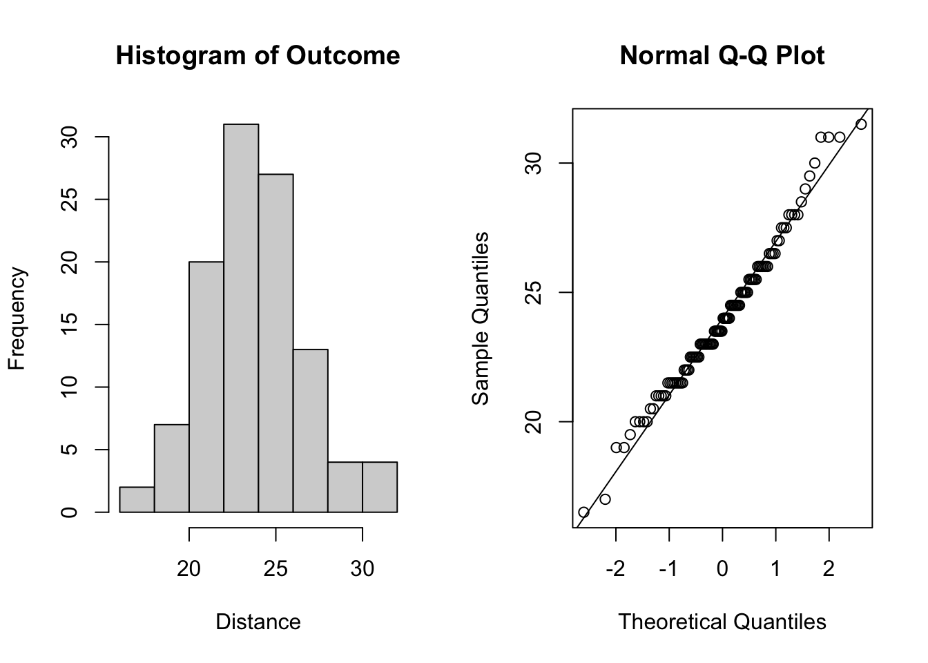

Figure 5.1: Plots for assessing normality of the outcome.

From the plots in Figure 5.1, we see that our outcomes appear to be normally distributed by the histogram. Additionally, we do not see any indication of non-normality in the data by the Q-Q plot as the sample quantiles do not deviate greatly from the theoretical quantiles of a normal distribution.

5.3.2 Notation and Model Specification

Assume we have \(n\) individuals observed at \(k\) common observation times.

Let:

• \(t_j\) be the \(j^{th}\) common assessment times, for \(j = 1, .., k\),
• \(Y_{ij}\) be the response of subject \(i\) at assessment time \(j\), for \(i = 1, ... ,n\) and \(j = 1, ... , k\), and
• \(\xx_{ij}\) be a \(p \times 1\) vector recording other covariates for subject \(i\) at time \(j\), for \(i = 1, ... ,n\) and \(j = 1, ... , k\).

We can write the observed data at each time point in matrix form. For each subject \(i = 1, ..., n\), we let \[ \bm{Y}_i = \begin{bmatrix} Y_{i1} \\ Y_{i2} \\ \vdots \\ Y_{ik} \\ \end{bmatrix} , \text{ and } \bm{X}_i = \begin{bmatrix} \bm{x}_{i1}^T \\ \bm{x}_{i2}^T \\ \vdots \\ \bm{x}_{ik}^T \\ \end{bmatrix} = \begin{bmatrix} x_{i11} & x_{i12}&\dots & x_{i1p} \\ x_{i21} & x_{i22}&\dots & x_{i2p} \\ \vdots & \vdots &\vdots & \vdots \\ x_{ik1} & x_{ik2}&\dots & x_{ikp} \end{bmatrix}. \]

To model the relationship between the outcome and other covariates, we can consider a linear regression model of the outcome of interest, \(Y_{ij}\) based on covariates \(x_{ij}\). \[ Y_{ij} = \beta_1x_{ij1} + \beta_2x_{ij2} + ... + \beta_px_{ijp} + e_{ij}, \tx{ for } j = 1, ..., k, \] where \(e_{ij}\) represents the random errors with mean zero. To include an intercept in this model, we can let \(x_{ij1} = 1\) for all subjects \(i\).

In practice, for longitudinal data, we model the mean of our outcome \(Y\). We assume that \(\bm{Y}_i\) conditional on \(\bm{X}_i\) follows a multivariate distribution: \[ \bm{Y}_i | \bm{X}_i \sim \N(\mu_i, \bm{\Sigma_i}), \] where \(\bm{\Sigma}_i = \cov(\YY_i | \XX_i)\) is a covariance matrix, whose form must be specified. The covariance matrix describes the relationship between pairs of observations within an individual. Specification of the correlation structure is discussed in the following section, Section 5.3.3.

With this notation, we can specify the corresponding linear model for \(\mu_i\), the mean of the outcome \(Y_i\) conditional on \(X_i\): \[ \mu_i = E(\bm{Y}_i | \bm{X}_i) = \bm{X}_i\bm{\beta} = \begin{bmatrix} \bm{x}_{i1}^T\bm{\beta} \\ \bm{x}_{i2}^T\bm{\beta} \\ \vdots \\ \bm{x}_{ik}^T\bm{\beta} \\ \end{bmatrix}. \]

We can then rewrite the multivariate normal assumption using the specified linear model as \[ \bm{Y}_i \sim \N(\bm{X}_i\bm{\beta}, \bm{\Sigma}_i). \] Again, to include an intercept in this model, we can let the first row of the matrix \(\XX\) be a row of ones. That is, \(x_{ij1} = 1\) for all subjects \(i\).

5.3.3 Correlation Structures

Unlike in most cross-sectional studies where we are working with data at a given “snapshot” in time, data in longitudinal studies are correlated due to the repeated samples taken on the same subjects. Thus, we need to model both the relationship between the outcome and the covariates and the correlation of the responses within an individual subject.

If we do not account for the correlation of responses within an individual, we may end up with

• incorrect conclusions and incorrect inferences on the parameters \(\bm{\beta}\),
• inefficient estimated of \(\bm{\beta}\), and/or
• more biases caused by missing data (Diggle et al. 2002).

Under a balanced longitudinal design with common observation times, we assume a common covariance matrix for all individuals, which can be written as \[ \bm{\Sigma}_i = \begin{bmatrix} \sigma_1^2 & \sigma_{12}& \dots & \sigma_{1k} \\ & \sigma_2^2 & \dots & \sigma_{2k} \\ & & \ddots & \vdots\\ & & & \sigma_k^2 \end{bmatrix}. \]

The diagonal elements in the above matrix represent the variances of the outcome \(Y\) at each time point while the off-diagonal elements represent the covariance between outcomes within a given individual at two different times. Estimating this covariance matrix can be problematic due to the large number of parameters we need to estimate. Hence, we consider different structures of covariance matrices to simplify it. We will refer to the collection of parameters in this variance-covariance matrix as \(\bm{\theta} = (\sigma_1^2, \sigma_2^2, ..., \sigma_k^2, \sigma_{12}, \sigma_{13}, ..., \sigma_{k-1,k})^T\) and can write the covariance matrix as a function of these parameters, \(\bm{\Sigma}(\bm{\theta})\).

We typically assume that the variance of the response does not change overtime, and thus we can write \[ \bm{\Sigma}_i = \sigma^2\bm{R}_i, \] where \(\bm{R}_i\) is referred to as a correlation matrix such that \[ \bm{R}_i = \begin{bmatrix} 1 & \rho_{12}& \dots & \rho_{1k} \\ & 1 & \dots & \rho_{2k} \\ & & \ddots & \vdots\\ & & & 1 \end{bmatrix}. \] This comes from the equation relating correlation and covariance, for example, \(\sigma_{12} = \sigma^2\rho_{12}\) when common variances are assumed.

We consider different structures of \(\bm{R}_i\) in our analyses and choose the most appropriate one based on the data. Commonly used correlation structures are:

• Unstructured Correlation, the least constrained structure: \[ \bm{R}_i = \begin{bmatrix} 1 & \rho_{12}& \dots & \rho_{1k} \\ & 1 & \dots & \rho_{2k} \\ & & \ddots & \vdots\\ & & & 1 \end{bmatrix}, \]

• Exchangeable Correlation, which is the simplest with only one parameter (excluding the variance \(\sigma^2\)) to estimate: \[ \bm{R}_i = \begin{bmatrix} 1 & \rho& \dots & \rho \\ & 1 & \dots & \rho \\ & & \ddots & \vdots\\ & & & 1 \end{bmatrix}, \]

• First-order Auto Regressive Correlation, which is sometimes referred to as “AR(1)” and is most suitable for evenly spaced observations where we see the correlation weakens as the time between observations gets larger: \[ \bm{R}_i = \begin{bmatrix} 1 & \rho & \rho^2 &\dots & \rho^{k-1} \\ & 1 & \rho &\dots & \rho^{k-2} \\ & & &\ddots & \vdots\\ & & & & 1 \end{bmatrix}, \]

• Exponential Correlation, where \(\rho_{jl} = \exp(-\phi|t_{ij} - t_{il}|)\) for some \(\phi > 0\), which collapses to AR(1) if observations are equally spaced.

We note that in practice, it is possible that the variance-covariance matrices differ among subjects, and the matrix may also depend on the covariates present in the data. More details about how to choose the appropriate structure will be discussed in Section 5.3.8.

5.3.4 Estimation

For convenience, let’s condense our notation to stack the response vectors and rewrite the linear model as \(\bm{Y}\sim N(\bm{X} \bm{\beta}, \Sigma)\) where \[ \bm{Y} = \begin{bmatrix} \bm{Y}_1 \\ \bm{Y}_2 \\ \vdots \\ \bm{Y}_n\\ \end{bmatrix} , \bm{X} = \begin{bmatrix} \bm{X}_1 \\ \bm{X}_2 \\ \vdots \\ \bm{X}_n\\ \end{bmatrix}, \text{ and } \bm{\Sigma} = \begin{bmatrix} \bm{\Sigma}_1 & 0 &\dots & 0 \\ & \bm{\Sigma}_2 &\dots & 0 \\ & &\ddots & \vdots\\ & & & \bm{\Sigma}_n \end{bmatrix}. \]

Under the multivariate normality assumptions, and with a fully specified distribution, one approach to estimate our regression parameters \(\beta\) and variance-covariance parameters \(\theta = (\sigma_1^2, \sigma_2^2, ..., \sigma_k^2, \sigma_{12}, \sigma_{13}, ..., \sigma_{k-1,k})^T\) is through maximum likelihood estimation.

The maximum likelihood estimate (MLE) of \(\beta\) is \[ \widehat{\bm{\beta}} = (\bm{X}^T\bm{\Sigma}^{-1}\bm{X})^{-1}\bm{X}^T\bm{\Sigma}^{-1}\bm{Y}. \]

This is a function of our variance-covariance matrix \(\bm{\Sigma}\) and thus a function of the parameters \(\theta\). As such, we can either estimate the parameters using profile likelihood or restricted maximum likelihood estimation (REML). The profile likelihood estimation is desirable because of the MLE’s large-sample properties. However, the MLEs of our variance and covariance parameters \(\bm{\theta}\) will be biased. The REML method was developed to overcome this issue. In general, the MLE (by the profile-likelihood approach) and REML estimates are not equal to each other for the regression parameters \(\bm{\beta}\), and thus we typically only use REML when estimating the variance and covariance parameters.

The MLE \(\widehat\beta\) has the asymptotic normality property. That is, \[ \hat{\bm{\beta}} \sim \N(\bm{\beta}, [\bm{X}^T\bm{\Sigma}^{-1}\bm{X}]^{-1}). \]

As \(\Sigma\) must be estimated, we typically estimate the asymptotic variance-covariance matrix as \[ \widehat{\text{asvar}}(\widehat{\bm{\beta}}) = (\bm{X}^T\widehat{\bm{\Sigma}}^{-1}\bm{X})^{-1}. \] We can use this to make inferences about regression parameters and perform hypothesis testing. For example, \[ \frac{\widehat{\beta}_j - \beta_j}{\sqrt{\widehat{\text{asvar}}}(\widehat{\beta}_j)} \dot{\sim} N(0,1), \] where \(\sqrt{\widehat{\text{asvar}}(\widehat{\beta}_j)} = (\bm{X}^T\widehat{\bm{\Sigma}}^{-1}\bm{X})^{-1}_{(jj)}\), i.e. the \((j,j)^{th}\) element of the asymptotic variance-covariance matrix.

5.3.5 Modelling in R

To fit a linear longitudinal model in R, we can use the gls() function from the nlme package. This function has a number of parameters, including

• model: a linear formula description of the form model = response ~ covariate1 + covariate2. Interaction effects can be specified using the form covariate1*covariate2 (NOTE: to add higher order terms, one must create a new variable in the original data set as operations like model = response ~ covariate1^2 will not be accepted in the model argument);
• correlation: the name of the within-group correlation structure, which may include corAR1 for the AR(1) structure, corCompSymm for the exchangeable structure, corExp for exponential structure, corSymm for unstructured, and others (see ?corClasses for other options). The default structure is an independent covariance structure;
• weights: an optional argument to allow for different marginal variances. For example, to allow for the variance of the responses to change for different discrete time/observation points, we can use weights = varIndent(form ~1 | factor(time)); and
• method: the name of the estimation method, where options include “ML” and “REML” (default).

To demonstrate the use of this package, we will apply the gls() function to the transformed (long form) dental data set.

Now, we can start to build our model, treating age as a categorical time variable. Define

• \(z_i\) to be the indicator for if subject \(i\) is male,
• \(t_{ij1}\) to be the indicator for if the age of individual \(i\) at observation \(j\) is 10,
• \(t_{ij2}\) to be the indicator for if the age of individual \(i\) at observation \(j\) is 12, and
• \(t_{ij3}\) to be the indicator for if the age of individual \(i\) at observation \(j\) is 14.

The main-effects model can be written as \[ \mu_{ij} = \beta_0 + \beta_1z_i + \beta_2t_{ij1} + \beta_3t_{ij2} + \beta_4t_{ij3}. \]

We will assume an unstructured working correlation structure for this model for illustrative purposes. In Section 5.3.8, we will describe how to choose the appropriate working correlation structure.

To fit a model and see the output, we can write:

fit1 <- gls(distance ~ factor(sex) + factor(age),
  data = dental_long,
  method = "ML",
  corr = corSymm(form = ~ 1 | subject) # unstructured
) 
# Note we are fitting the model using Maximum
# likelihood estimation and with no interactions (main effects only).

summary(fit1) # see the output of the fit

## Generalized least squares fit by maximum likelihood
##   Model: distance ~ factor(sex) + factor(age) 
##   Data: dental_long 
##        AIC      BIC    logLik
##   450.3138 482.4993 -213.1569
## 
## Correlation Structure: General
##  Formula: ~1 | subject 
##  Parameter estimate(s):
##  Correlation: 
##   1     2     3    
## 2 0.591            
## 3 0.623 0.532      
## 4 0.464 0.674 0.700
## 
## Coefficients:
##                   Value Std.Error  t-value p-value
## (Intercept)   20.833863 0.6235854 33.40980  0.0000
## factor(sex)M   2.280355 0.7461323  3.05623  0.0029
## factor(age)10  0.981481 0.3976474  2.46822  0.0152
## factor(age)12  2.462963 0.3820559  6.44660  0.0000
## factor(age)14  3.907407 0.4554203  8.57978  0.0000
## 
##  Correlation: 
##               (Intr) fct()M fc()10 fc()12
## factor(sex)M  -0.709                     
## factor(age)10 -0.319  0.000              
## factor(age)12 -0.306  0.000  0.405       
## factor(age)14 -0.365  0.000  0.661  0.682
## 
## Standardized residuals:
##         Min          Q1         Med          Q3         Max 
## -2.74011685 -0.70682170 -0.05118776  0.57834032  2.43026224 
## 
## Residual standard error: 2.231372 
## Degrees of freedom: 108 total; 103 residual

Under the assumption that the working correlation structure is unstructured, we can assess which variables impact the outcome (our distance measurement). In the summary of the coefficients for our model, we have very small \(p\)-values for our sex variable (\(p\) = 0.0029), indicating that there is a difference in distance measurements between boys and girls enrolled in the study, when controlling for the time effect. Additionally, the \(p\)-values indicating the timings of the observations are small, with increasingly large coefficients, providing evidence of a possible time trend in our data. These \(p\)-values come from \(t\)-tests for the null hypothesis that the coefficient of interest is zero.

Note: similar to linear regression models, if you would like to remove the intercept in the model, we would use the formula distance ~ factor(sex) + factor(age) - 1 when fitting the model.

5.3.6 Hypothesis Testing

Suppose we want to see if the time trend differs between the sexes of children enrolled in the study. To formally test if there is a common time-trend between groups (sex), we can fit a model including an interaction term and perform a hypothesis test. The interaction model can be written as \[ \mu_{ij} = \beta_0 + \beta_1z_i + \beta_2t_{ij1} + \beta_3t_{ij2} + \beta_4t_{ij3} + \beta_5z_it_{ij1} + \beta_6z_it_{ij2} + \beta_7z_it_{ij3}. \]

We fit the required model using the following code, and for now assume an unstructured correlation structure:

fit2 <- gls(distance ~ factor(sex) * factor(age),
  data = dental_long,
  method = "ML",
  corr = corSymm(form = ~ 1 | subject) # unstructured 
) 
# Note we are fitting the model using Maximum
# likelihood estimation and with main effects and interactions (by using *).

summary(fit2) # see the output of the fit

## Generalized least squares fit by maximum likelihood
##   Model: distance ~ factor(sex) * factor(age) 
##   Data: dental_long 
##       AIC     BIC    logLik
##   448.377 488.609 -209.1885
## 
## Correlation Structure: General
##  Formula: ~1 | subject 
##  Parameter estimate(s):
##  Correlation: 
##   1     2     3    
## 2 0.580            
## 3 0.637 0.553      
## 4 0.516 0.753 0.705
## 
## Coefficients:
##                                Value Std.Error   t-value p-value
## (Intercept)                21.181818 0.6922613 30.598009  0.0000
## factor(sex)M                1.693182 0.8992738  1.882832  0.0626
## factor(age)10               1.045455 0.6344963  1.647692  0.1026
## factor(age)12               1.909091 0.5899117  3.236231  0.0016
## factor(age)14               2.909091 0.6812865  4.269996  0.0000
## factor(sex)M:factor(age)10 -0.107955 0.8242348 -0.130975  0.8961
## factor(sex)M:factor(age)12  0.934659 0.7663178  1.219675  0.2255
## factor(sex)M:factor(age)14  1.684659 0.8850171  1.903533  0.0598
## 
##  Correlation: 
##                            (Intr) fct()M fc()10 fc()12 fc()14 f()M:()10
## factor(sex)M               -0.770                                      
## factor(age)10              -0.458  0.353                               
## factor(age)12              -0.426  0.328  0.431                        
## factor(age)14              -0.492  0.379  0.729  0.658                 
## factor(sex)M:factor(age)10  0.353 -0.458 -0.770 -0.332 -0.561          
## factor(sex)M:factor(age)12  0.328 -0.426 -0.332 -0.770 -0.507  0.431   
## factor(sex)M:factor(age)14  0.379 -0.492 -0.561 -0.507 -0.770  0.729   
##                            f()M:()12
## factor(sex)M                        
## factor(age)10                       
## factor(age)12                       
## factor(age)14                       
## factor(sex)M:factor(age)10          
## factor(sex)M:factor(age)12          
## factor(sex)M:factor(age)14  0.658   
## 
## Standardized residuals:
##         Min          Q1         Med          Q3         Max 
## -2.65921430 -0.63297787 -0.08229677  0.63779995  2.39046391 
## 
## Residual standard error: 2.209299 
## Degrees of freedom: 108 total; 100 residual

To test the difference in time-trends between groups (sex), we test if the last three coefficients (\(\beta_5\), \(\beta_6\), and \(\beta_7\), that are associated with the interaction terms in our model) are all equal to zero. We are testing \(H_0: \beta_5 = \beta_6 = \beta_7 = 0\) vs \(H_a\): at least one of these coefficients is non-zero. To do so, we need to define a matrix. This matrix has one column for each estimated coefficient (including the intercept) and one row for each coefficient in the hypothesis test. As such, for this particular hypothesis test, let’s define the matrix \[ \bm{L} = \begin{bmatrix} 0 & 0 & 0 & 0 & 0 & 1 & 0 & 0 \\ 0 & 0 & 0 & 0 & 0 & 0 & 1 & 0 \\ 0 & 0 & 0 & 0 & 0 & 0 & 0 & 1 \\ \end{bmatrix}, \] which will be used to calculate our Wald test statistic \((\bm{L}\widehat{\bm{\beta}})^T[\bm{L}\widehat{\text{asvar}}(\widehat{\bm{\beta}})\bm{L}^T]^{-1}(\bm{L}\widehat{\bm{\beta}})\). This test statistic follows a chi-squared distribution with the degree of freedom equal to the rank of the matrix \(\bm{L}\) (which is 3 in this case).

To perform this hypothesis test in R, we do the following:

L <- rbind(
  c(0, 0, 0, 0, 0, 1, 0, 0),
  c(0, 0, 0, 0, 0, 0, 1, 0),
  c(0, 0, 0, 0, 0, 0, 0, 1)
) # create L matrix as above

betahat <- fit2$coef # get estimated beta hats from the model

asvar <- fit2$varBeta # get the estimated covariances from the model

# calculate test statistic using given formula
waldtest_stat <- t(L %*% betahat) %*% solve(L %*% asvar %*% t(L)) %*% (L %*% betahat)
waldtest_stat

##         [,1]
## [1,] 8.60252

To get a \(p\)-value for this test, we perform the following:

pval <- 1 - pchisq(waldtest_stat, 3) # test stat follows chi-squared 3 in this case
pval

##            [,1]
## [1,] 0.03507014

We have a small \(p\)-value, which tells us that we have sufficient evidence against \(H_0\). That is, we have evidence to suggest that the time trends vary by sex, and the model (fit2) with the interactions is more appropriate.

We can also do a likelihood ratio test (LRT) as these models are nested within each other (i.e., all parameters in fit1 are also present in fit2, so fit1 is nested in fit2). The test statistic is \(\Lambda = -2(l_2-l_1)\) where \(l_2\) is the log-likelihood of fit2 (the bigger model), and \(l_1\) is the log-likelihood of fit1 (nested model). The degree of freedom is the same as in the chi-squared test. Note that models both must be fit using maximum likelihood (ML argument) to perform the LRT for model parameters, and be fit with the same correlation structure.

anova(fit1, fit2)

##      Model df      AIC      BIC    logLik   Test  L.Ratio p-value
## fit1     1 12 450.3138 482.4993 -213.1569                        
## fit2     2 15 448.3770 488.6090 -209.1885 1 vs 2 7.936725  0.0473

Again, we have a small \(p\)-value and come to the same conclusion as in the Wald test, which is to reject the null and use the model with the interaction terms.

We could additionally test if there was a difference in distance at baseline between sexes (\(H_0: \beta_1 = 0\)) in a similar manner, or by looking at the \(p\)-value in the model summary for the sex coefficient.

Note: If we had come to the conclusion that the time trends were the same among groups, the same methods could be used to test the hypothesis that there is no time effect (\(H_0: \beta_2 = \beta_3 = \beta_4 = 0\)) or the hypothesis that there is no difference in mean outcome by sex (\(H_0: \beta_1 = 0\)).

We again emphasize that the results can differ based on the chosen correlation structure.

5.3.7 Population Means

Using the asymptotic results of our MLE for \(\bm{\beta}\), we can estimate the population means for different subgroups in the data, and/or at different time points. For example, suppose we would like to know the mean distance at age 14 for males in the study, i.e. we want to estimate \(\mu = \beta_0 + \beta_1 + \beta_4\). We can define a vector \[ \bm{L} = [1,1,0,0,1] \] to obtain the estimate \[ \widehat{\mu} = \bm{L}\widehat{\bm{\beta}} = \widehat{\beta_0} + \widehat{\beta_1} + \widehat{\beta_4}, \] along with its standard error \[ se(\widehat{\mu}) = \sqrt{\bm{L}\widehat{\text{asvar}}(\widehat{\bm{\beta}})\bm{L}^T}. \]

The code to obtain these estimates is as follows:

betahat <- fit1$coef # get estimated betas from model 1
varbeta <- fit1$varBeta # get estimated variance covariance matrix from model 1

L <- matrix(c(1, 1, 0, 0, 1), nrow = 1) # set up row vector L

muhat <- L %*% betahat # calculate estimated mean
se <- sqrt(L %*% varbeta %*% t(L)) # calculated estimated variance

muhat

##          [,1]
## [1,] 27.02163

se

##           [,1]
## [1,] 0.5345687

With these quantities, we can also construct a 95% confidence interval for the mean as \(\widehat{\mu} \pm 1.960*se(\widehat{\mu})\).

CI_l <- muhat - 1.960 * se # calculate lower CI bound
CI_u <- muhat + 1.960 * se # calculate upper CI bound

print(paste("(", round(CI_l, 3), ", ", round(CI_u, 3), ")", sep = "")) # output the CI

## [1] "(25.974, 28.069)"

That is, we are 95% confident that the mean outcome for 14 year old male subjects falls between (25.974, 28.069).

Similar calculations can be performed for other population means of interest.

5.3.8 Selecting a Correlation Structure

In the previous examples, for illustrative purposes we assumed an unstructured correlation structure. It is likely that in practice we can use a simpler structure, and thus we need to perform hypothesis tests to select the appropriate structure.

To select a correlation structure, we use the REML method instead of the ML method when fitting our models, since maximum likelihood estimation is biased for our covariance parameters. Our goal is to choose the simplest correlation structure while maintaining an adequate model fit.

Some correlation structures are nested within each other (meaning you can chose parameters such that one simplifies into the other), and we can perform likelihood ratio tests to assess the adequacy of the correlation structures. For example, the exchangeable correlation structure is nested within the unstructured covariance structure. As such, we can perform a hypothesis test of \(H_0\): The simpler correlation structure (exchangeable) fits as well as the more complex structure (unstructured).

To do this test, we fit our model (we will continue using the model including interactions here) using restricted maximum likelihood estimation and perform the LRT.

fit1_unstructured <- gls(distance ~ factor(sex)*factor(age),
  data = dental_long,
  method = "REML",
  corr = corSymm(form = ~ 1 | subject)
) # subject is the variable indicating
# repeated measures. Unstructured corr

fit1_exchangeable <- gls(distance ~ factor(sex)*factor(age),
  data = dental_long,
  method = "REML",
  corr = corCompSymm(form = ~ 1 | subject)
) # subject is the variable indicating
# repeated measures. Exchangeable corr

anova(fit1_unstructured, fit1_exchangeable)

##                   Model df      AIC      BIC    logLik   Test  L.Ratio p-value
## fit1_unstructured     1 15 445.7642 484.8417 -207.8821                        
## fit1_exchangeable     2 10 443.4085 469.4602 -211.7043 1 vs 2 7.644354   0.177

We have a large \(p\)-value and thus fail to reject the null hypothesis. That is, we will use the exchangeable correlation structure as it is simpler and fits as well.

For non-nested correlation structures like AR(1) and exchangeable, we can use AIC or BIC to assess the fit, where a smaller AIC/BIC indicates a better fit. AIC and BIC are similar, but achieve different goals in model selection and one is not strictly preferred over the other. In fact, they are often used for model selection together. For the purposes of this analysis, we choose to only show the results for AIC, as using BIC will yield similar results. More information on AIC and BIC can be found here.

fit1_ar1 <- gls(distance ~ factor(sex)*factor(age),
  data = dental_long,
  method = "REML",
  corr = corAR1(form = ~ 1 | subject)
) # subject is the variable indicating
# repeated measures. Exchangeable corr

AIC(fit1_exchangeable)

## [1] 443.4085

AIC(fit1_ar1)

## [1] 454.5472

We see that the model using an exchangeable correlation structure has a smaller AIC, which indicates a better fit. In this case, we would choose the exchangeable correlation structure over the auto-regressive structure. We note that similar tests can be performed for other correlation structures, but are omitted for the purposes of this example.

5.3.9 Model Fitting Procedure

We start the model fitting procedure by

1. reading in and cleaning the data, then

2. checking model assumptions assumptions, including checking if

   • the outcome is normally distributed (see Section 5.3.1),

   • observations are taken at the same times for all subjects, and

   • there are no missing observations in the data set.

If the above conditions are satisfied, we can start fitting/building a model. It is usually recommended to

3. focus on the time trend of the response (assess if we should have a continuous or discrete time variable, need higher-order terms, and/or interactions), then

4. find the appropriate covariance structure, then

5. consider variable selection.

This process can be done iteratively on steps 3 - 5 until a final model is chosen based on the appropriate statistical tests and the scientific question of interest.

We note that the model building process can be done with the consultation of expert opinions, if available, to include “a priori” variables in the model that should be included regardless of statistical significance.

5.3.10 Example

We follow the model fitting procedure presented in 5.3.9 to answer a different research question on a new data set. The data set tlc, which is stored in a text file in the “data” folder, consists of 100 children who were randomly assigned to chelation treatment with the addition of either succimer or placebo. Four repeated measurements of blood lead levels were obtained at baseline (week 0), week 1, week 4, and week 6. We note this data set has the same observation pattern for all individuals in the study, and no missing observations, which is a requirement for the linear model.

The research question of interest is whether there is a difference in the mean blood lead level over time between the succimer (which we we will refer to as the treatment group) or placebo group.

Step 1: Data Read in and Cleaning

We first read in the data and rename the columns. We also rename the Group variable values to be more clear, where group “A” corresponds to succimer treatment group and group “P” corresponds to the placebo.

# read in the data set
tlc <- read.table("data/tlc.txt")

# rename the columns
colnames(tlc) <- c("ID", "Group", "week0", "week1", "week4", "week6")

# rename the P and A groups to Placebo and Succimer
tlc[tlc$Group == "P", "Group"] <- "Placebo"
tlc[tlc$Group == "A", "Group"] <- "Succimer"

and convert our data to long-form

# reshape the data into long form
tlc_long <- reshape(
  data = tlc, # original data in wide form
  direction = "long", # changing from wide TO long
  idvar = "ID", # name of variable indicating unique
  # subjects in wide form data set
  varying = c("week0", "week1", "week4", "week6"), # name
  # of variables in which outcomes recorded
  v.names = "bloodlev", # assigning a new name to the outcome
  times = c(0,1,4,6), # time points in which the above
  # outcomes were recorded
  timevar = "week"
) # name of the time variable we're using

# order the data by subject ID and then by week
tlc_long <- tlc_long[order(tlc_long$ID, tlc_long$week), ]

# look at the first 10 observations
head(tlc_long, 10)

##     ID    Group week bloodlev
## 1.0  1  Placebo    0     30.8
## 1.1  1  Placebo    1     26.9
## 1.4  1  Placebo    4     25.8
## 1.6  1  Placebo    6     23.8
## 2.0  2 Succimer    0     26.5
## 2.1  2 Succimer    1     14.8
## 2.4  2 Succimer    4     19.5
## 2.6  2 Succimer    6     21.0
## 3.0  3 Succimer    0     25.8
## 3.1  3 Succimer    1     23.0

Step 2: Checking Model Assumptions

Now that the data is in long form, we can begin to explore the data. We first assess the normality assumption of the outcome of interest, bloodlev. We do this by looking at the distribution of the outcome and by creating a Q-Q plot.

par(mfrow = c(1, 2)) # set graphs to be arranged in one row and two columns

# histogram of outcome
hist(tlc_long$bloodlev, xlab = "Blood lead level", main = "Histogram of Outcome")

# Q-Q plot and line
qqnorm(tlc_long$bloodlev) # plot quantiles against normal distribution
qqline(tlc_long$bloodlev) # add line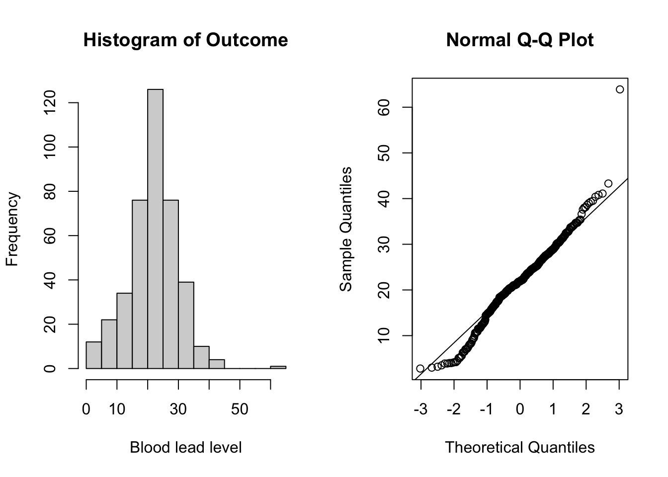

Figure 5.2: Plots for assessing normality of the outcome (blood lead level).

From the plots in Figure 5.2, we do not see evidence of non-normality and can continue with the linear model. See Section 5.3.1 for more details on assessing normality.

Step 3: Assessing Time Trend

The next step is to assess the time trend. We can first explore the data by looking at the average profile across the two groups and see if there is a linear trend, or if we need to consider higher-order terms. We can do this using the xyplot() function from the lattice package

xyplot(bloodlev ~ week | factor(Group), # plotting bloodlev over time, by group
data = tlc_long,
xlab = "time (weeks)", ylab = "Blood lead levels", # axis labels
main = "Plot of individual blood lead levels by treatment group", # title
panel = function(x,y){
panel.xyplot(x, y, type = "p") # plots individual values 
panel.linejoin(x,y, fun = mean, horizontal = F, lwd = 2, col = 1)}) # plots mean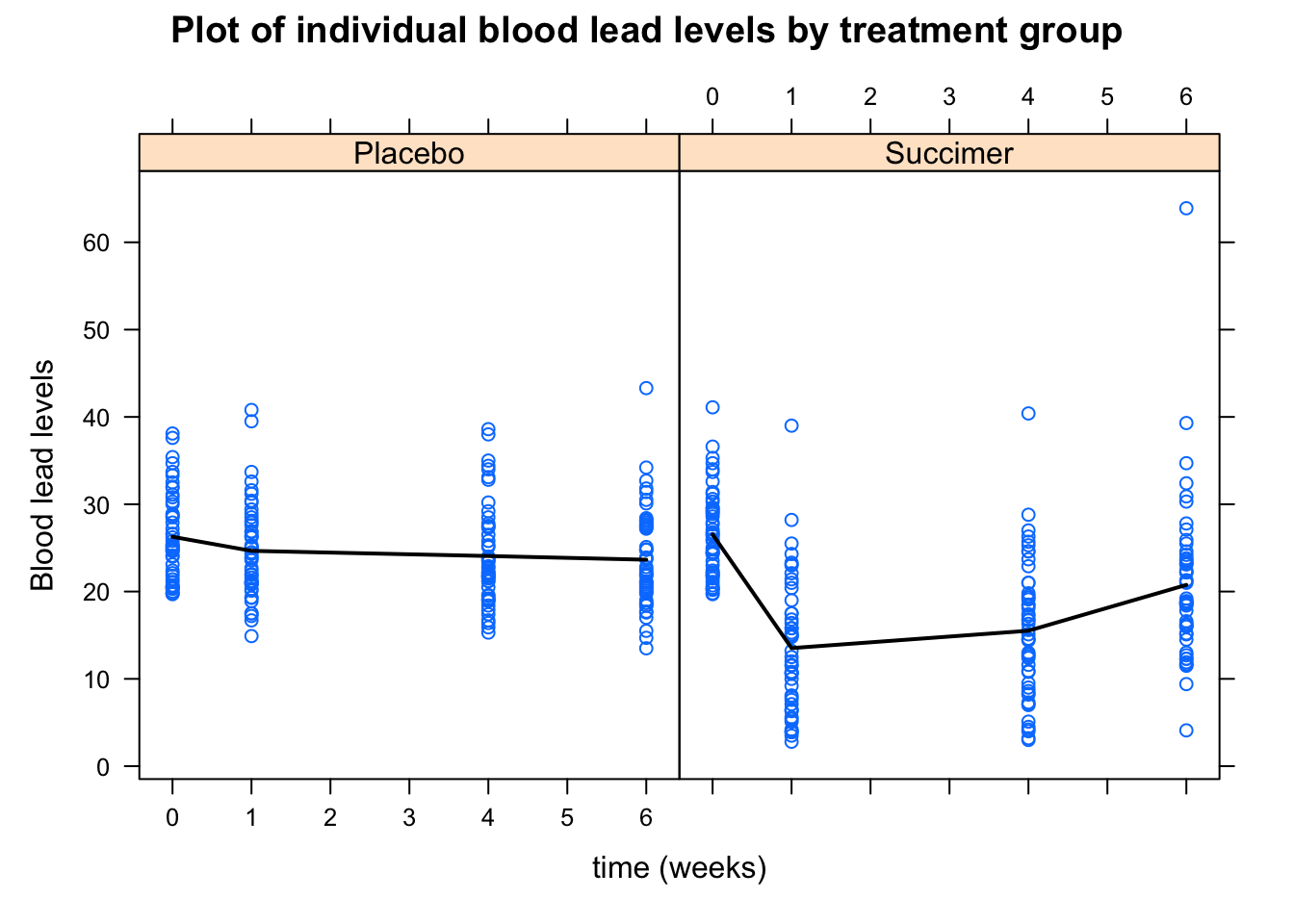

Figure 5.3: Plot of individual blood lead levels stratified by treatment group. Dark line represents mean blood level at each observation times.

From the plot in Figure 5.3, there does not appear to be a linear time trend, particularly for the succimer group. There also appears to be a difference in trend between the succimer and placebo groups. As such, we should consider transformations or higher-order terms for time (such as quadratic (squared) time effects for the non-linear trend) and also interaction terms between the group and time variables (to account for differences in trend by group).

In this example, we will not categorize the time trend and treat it as a continuous covariate. This allows us to quantify the effect of a one unit change of time on the outcome. This is a different way of looking at time, as opposed to the working example in the module that categorized time. Whether or not to treat time as continuous or categorical will depend on the research goal and the data.

The model we start with is a linear trend model for the marginal mean, written as \[ \mu_{ij} = \beta_0 + \beta_1\text{Group}_{ij} + \beta_2 \text{week}_{ij} + \beta_3\text{Group}_i\text{week}_{ij} . \] Here we have an individual group effect (\(\beta_1\)) that allows the groups to differ at baseline, a linear time effect (\(\beta_2\) ) for our week variable, and an interaction term that allows the trends to differ by group (\(\beta_3\)).

We can fit our model using the gls() function using the ML method, and assume an unstructured correlation structure.

fit1_tlc <- gls(bloodlev ~ Group*week,  method = "ML", # maximum likelihood method
                data = tlc_long, corr = corSymm(form = ~1 | ID)) # unstructured cor

We compare this model to one that includes a quadratic time effect (and higher-order interactions), written as \[ \mu_{ij} = \beta_0 + \beta_1\text{Group}_{ij} + \beta_2 \text{week}_{ij} + \beta_3\text{week}^2_{ij} + \beta_4\text{Group}_i\text{week}_{ij} + \beta_5\text{Group}_i\text{week}^2_{ij}. \] Here we have an individual group effect (\(\beta_1\)) that allows the groups to differ at baseline, a linear and quadratic effect (\(\beta_2\) and \(\beta_3\)) for our time variable (week) that allows for non-linear trends, and two interaction terms that allow the trends to differ by group (\(\beta_4\) and \(\beta_5\)).

To fit the above model, we need to create an additional variable in our data set for the squared time variable. To do so, we perform the following:

tlc_long$weeksq <- (tlc_long$week)^2 # create squared week variable

Then, we fit a model with the squared time variable, to see if the squared time variable is necessary in the model and perform a LRT:

fit2_tlc <- gls(bloodlev ~ Group*week + Group*weeksq , method = "ML", #no squared week term
                data = tlc_long, corr = corSymm(form = ~1 | ID))
                #unstructured correlation again

# perform hypothesis test to see if linear model (fit1) fits 
# as well as new model with squared time terms (fit2)
anova(fit1_tlc, fit2_tlc)

##          Model df      AIC      BIC    logLik   Test  L.Ratio p-value
## fit1_tlc     1 11 2593.256 2637.162 -1285.628                        
## fit2_tlc     2 13 2554.344 2606.233 -1264.172 1 vs 2 42.91194  <.0001

As the \(p\)-value here is very small (\(p<0.0001\)), we reject the null hypothesis that the model without the squared week term fits as well as the model that includes it.

We can also investigate higher-order terms in a similar manner, including cubic transformations of the week variable. The model can be written as

\[ \begin{aligned} \mu_{ij} = \beta_0 + \beta_1\text{Group}_{ij} + &\beta_2 \text{week}_{ij} + \beta_3\text{week}^2_{ij} + \beta_4\text{week}^3 + \beta_5\text{Group}_i\text{week}_{ij} +\\ &\beta_6\text{Group}_i\text{week}^2_{ij} + \beta_7\text{Group}_i\text{week}_{ij}^3. \end{aligned} \] We first create a cubic term:

tlc_long$weekcb <- (tlc_long$week)^3 # create cubed week variable

We can again fit this model using the gls() function, specifying the ML method and again assuming an unstructured correlation structure:

fit3_tlc <- gls(bloodlev ~ Group*week + Group*weeksq + Group*weekcb,  method = "ML",
                data = tlc_long, corr = corSymm(form = ~1 | ID))

# perform hypothesis test to see if model with squared time term (fit2) fits 
# as well as new model with cubic time terms (fit3)
anova(fit3_tlc, fit2_tlc)

##          Model df      AIC      BIC    logLik   Test  L.Ratio p-value
## fit3_tlc     1 15 2481.445 2541.317 -1225.722                        
## fit2_tlc     2 13 2554.344 2606.233 -1264.172 1 vs 2 76.89944  <.0001

We again reject the null hypothesis and conclude that we should have cubic terms of our week variable in the model. As such, we continue model building with the third model that contains both squared and cubic transformations of our time variable (week). More details on such tests can be found in Section 5.3.6, and we note that analysts can consider other transformations of time, and refer them to (Fitzmaurice, Laird, and Ware 2011) for further discussion and examples.

Step 4: Selecting a Covariance Structure

The next step is to select a covariance structure, as detailed in Section 5.3.8. Note that we must re-fit the model using the REML method as we are conducting inference about the covariance structure.

fit3_tlc_REML <- gls(bloodlev ~ Group*week + Group*weeksq + Group*weekcb,  
                     method = "REML", data = tlc_long, 
                     corr = corSymm(form = ~1 | ID)) # unstructured cov

We perform hypothesis test to see if we can simplify the correlation structure further. For this example, we will be considering the following correlation structures: independent, exchangeable, and AR(1). We recognize there are other structures that could also be explored, but consider these structures for the purposes of this example. We see if the simplest correlation structure, the independence structure, fits as well as the current model (unstructured) by a likelihood ratio test. We can perform a LRT because the independence structure is “nested” in unstructured, meaning that we can write the independent structure in terms of the unstructured. Details on what to do for un-nested structures are discussed in 5.3.8.

fit3_tlc_REML_ind <- gls(bloodlev ~ week*Group + weeksq*Group + weekcb*Group,  
                     method = "REML", data = tlc_long) # default cor: independent

#perform LRT
anova(fit3_tlc_REML, fit3_tlc_REML_ind)

## Warning in nlme::anova.lme(object = fit3_tlc_REML, fit3_tlc_REML_ind): fitted
## objects with different fixed effects. REML comparisons are not meaningful.

##                   Model df      AIC      BIC    logLik   Test  L.Ratio p-value
## fit3_tlc_REML         1 15 2497.949 2557.517 -1233.974                        
## fit3_tlc_REML_ind     2  9 2670.572 2706.314 -1326.286 1 vs 2 184.6236  <.0001

We reject the null hypothesis that the model with the independent correlation structure fits as well as the unstructured model. We note that we come to a similar conclusion when assessing the AIC for each model.

AIC(fit3_tlc_REML)

## [1] 2497.949

AIC(fit3_tlc_REML_ind)

## [1] 2670.572

The model with an unstructured correlation structure has a much lower AIC, indicating a better fit than the independent structure.

We next see if an exchangeable correlation structure will be sufficient. We re-fit the model again with an exchangeable correlation structure, and compare it to the unstructured model.

fit3_tlc_REML_exch <- gls(bloodlev ~ Group*week + Group*weeksq + Group*weekcb,  
                     method = "REML", data = tlc_long,
                     corr = corCompSymm(form=~1 | ID)) # exchangeable

#perform LRT
anova(fit3_tlc_REML, fit3_tlc_REML_exch)

##                    Model df      AIC      BIC    logLik   Test  L.Ratio p-value
## fit3_tlc_REML          1 15 2497.949 2557.517 -1233.974                        
## fit3_tlc_REML_exch     2 10 2506.938 2546.651 -1243.469 1 vs 2 18.98944  0.0019

We again reject the null hypothesis and conclude the unstructured model fits better. We note that we come to a similar conclusion when assessing the AIC for each model.

AIC(fit3_tlc_REML)

## [1] 2497.949

AIC(fit3_tlc_REML_exch)

## [1] 2506.938

We can next consider an AR(1) model for the correlation structure.

fit3_tlc_REML_ar1 <- gls(bloodlev ~ Group*week + Group*weeksq + Group*weekcb,  
                     method = "REML", data = tlc_long,
                     corr = corAR1(form=~1 | ID)) # AR(1)

#perform LRT
anova(fit3_tlc_REML, fit3_tlc_REML_ar1)

##                   Model df      AIC      BIC    logLik   Test  L.Ratio p-value
## fit3_tlc_REML         1 15 2497.949 2557.517 -1233.974                        
## fit3_tlc_REML_ar1     2 10 2518.948 2558.660 -1249.474 1 vs 2 30.99904  <.0001

We reject this null hypothesis as well. We again come to a similar conclusion when assessing the AIC for each model.

AIC(fit3_tlc_REML)

## [1] 2497.949

AIC(fit3_tlc_REML_ar1)

## [1] 2518.948

We try one final structure, the exponential correlation structure.

fit3_tlc_REML_exp <- gls(bloodlev ~ Group*week + Group*weeksq + Group*weekcb,  
                     method = "REML", data = tlc_long,
                     corr = corExp(form=~1 | ID)) # exponential

#perform LRT
anova(fit3_tlc_REML, fit3_tlc_REML_exp)

##                   Model df      AIC      BIC    logLik   Test  L.Ratio p-value
## fit3_tlc_REML         1 15 2497.949 2557.517 -1233.974                        
## fit3_tlc_REML_exp     2 10 2518.948 2558.660 -1249.474 1 vs 2 30.99904  <.0001

We again reject the null hypothesis. Checking the AIC:

AIC(fit3_tlc_REML)

## [1] 2497.949

AIC(fit3_tlc_REML_exp)

## [1] 2518.948

We obtain the same conclusion that the unstructured correlation structure fits better. Based on these tests, we decide to stay with the unstructured correlation structure as there is no evidence that we are able to simplify it into any of the above options.

Step 5: Selecting Variables

Now that we have the form of the time trend and the correlation structure chosen, we consider variable selection in our model, meaning we attempt to simplify the model as much as possible by reducing the number of variables in our model. We first re-fit the model using the ML method as we are no longer concerned about estimation of the correlation structure.

fit_tlc_full <- gls(bloodlev ~ Group*week + Group*weeksq + Group*weekcb,  method = "ML",
                data = tlc_long, corr = corSymm(form = ~1 | ID))

We can first investigate if the treatment groups’ blood lead levels differ at baseline. We can do this by performing a hypothesis test to see if the Group term is necessary in the model, or equivalently if \(\beta_1 = 0\) in the model

\[ \begin{aligned} \mu_{ij} = \beta_0 + \beta_1\text{Group}_{ij} + &\beta_2 \text{week}_{ij} + \beta_3\text{week}^2_{ij} + \beta_4\text{week}^3 + \beta_5\text{Group}_i\text{week}_{ij} +\\ &\beta_6\text{Group}_i\text{week}^2_{ij} + \beta_7\text{Group}_i\text{week}_{ij}^3. \end{aligned} \] The results of this hypothesis test are given in the model summary, which we can view using the summary() function on our model:

summary(fit_tlc_full)

## Generalized least squares fit by maximum likelihood
##   Model: bloodlev ~ Group * week + Group * weeksq + Group * weekcb 
##   Data: tlc_long 
##        AIC      BIC    logLik
##   2481.445 2541.317 -1225.722
## 
## Correlation Structure: General
##  Formula: ~1 | ID 
##  Parameter estimate(s):
##  Correlation: 
##   1     2     3    
## 2 0.596            
## 3 0.582 0.769      
## 4 0.536 0.552 0.551
## 
## Coefficients:
##                           Value Std.Error   t-value p-value
## (Intercept)           26.272000 0.9374730 28.024274  0.0000
## GroupSuccimer          0.268000 1.3257870  0.202144  0.8399
## week                  -2.203767 1.2319182 -1.788890  0.0744
## weeksq                 0.651250 0.4519714  1.440910  0.1504
## weekcb                -0.059483 0.0454380 -1.309111  0.1913
## GroupSuccimer:week   -16.253733 1.7421954 -9.329455  0.0000
## GroupSuccimer:weeksq   5.293000 0.6391840  8.280870  0.0000
## GroupSuccimer:weekcb  -0.445267 0.0642590 -6.929250  0.0000
## 
##  Correlation: 
##                      (Intr) GrpScc week   weeksq weekcb GropSccmr:wk
## GroupSuccimer        -0.707                                         
## week                 -0.436  0.308                                  
## weeksq                0.386 -0.273 -0.964                           
## weekcb               -0.355  0.251  0.891 -0.978                    
## GroupSuccimer:week    0.308 -0.436 -0.707  0.682 -0.630             
## GroupSuccimer:weeksq -0.273  0.386  0.682 -0.707  0.691 -0.964      
## GroupSuccimer:weekcb  0.251 -0.355 -0.630  0.691 -0.707  0.891      
##                      GrpSccmr:wks
## GroupSuccimer                    
## week                             
## weeksq                           
## weekcb                           
## GroupSuccimer:week               
## GroupSuccimer:weeksq             
## GroupSuccimer:weekcb -0.978      
## 
## Standardized residuals:
##        Min         Q1        Med         Q3        Max 
## -2.5390445 -0.7040965 -0.1513186  0.5596352  6.5735988 
## 
## Residual standard error: 6.562311 
## Degrees of freedom: 400 total; 392 residual

Under the “coefficients” section of the summary, the estimated coefficients along with their standard errors, \(t\)-values, and \(p\)-values for the hypothesis test that that coefficient is equal to zero are presented. For the GroupSuccimer variable that indicates if the treatment group is succimer or not, the \(p\)-value for the hypothesis test is 0.8399, which is large. This indicates that we fail to reject the null hypothesis of \(H_0: \beta_1 = 0\) and conclude that we do not need to keep this variable in the model, and the treatment groups’ mean blood lead level do not differ at baseline.

We re-fit the model without this variable. In this case, we need to write out individual terms as using * will include the non-interaction terms as well.

fit_tlc_full2 <- gls(bloodlev ~ week + weeksq + weekcb + Group:week + 
                    Group:weeksq + Group:weekcb,  
                    method = "ML",
                    data = tlc_long, corr = corSymm(form = ~1 | ID))
summary(fit_tlc_full2)

## Generalized least squares fit by maximum likelihood
##   Model: bloodlev ~ week + weeksq + weekcb + Group:week + Group:weeksq +      Group:weekcb 
##   Data: tlc_long 
##        AIC      BIC    logLik
##   2479.487 2535.367 -1225.743
## 
## Correlation Structure: General
##  Formula: ~1 | ID 
##  Parameter estimate(s):
##  Correlation: 
##   1     2     3    
## 2 0.596            
## 3 0.582 0.769      
## 4 0.536 0.552 0.551
## 
## Coefficients:
##                           Value Std.Error   t-value p-value
## (Intercept)           26.406000 0.6621227  39.88082  0.0000
## week                  -2.280478 1.1705109  -1.94828  0.0521
## weeksq                 0.676158 0.4342959   1.55691  0.1203
## weekcb                -0.061792 0.0439236  -1.40680  0.1603
## week:GroupSuccimer   -16.100310 1.5661533 -10.28016  0.0000
## weeksq:GroupSuccimer   5.243185 0.5890086   8.90171  0.0000
## weekcb:GroupSuccimer  -0.440650 0.0599862  -7.34585  0.0000
## 
##  Correlation: 
##                      (Intr) week   weeksq weekcb wk:GrS wks:GS
## week                 -0.324                                   
## weeksq                0.283 -0.961                            
## weekcb               -0.260  0.883 -0.976                     
## week:GroupSuccimer    0.000 -0.669  0.650 -0.597              
## weeksq:GroupSuccimer  0.000  0.641 -0.678  0.666 -0.959       
## weekcb:GroupSuccimer  0.000 -0.585  0.661 -0.683  0.875 -0.975
## 
## Standardized residuals:
##        Min         Q1        Med         Q3        Max 
## -2.5278255 -0.7018094 -0.1484155  0.5498241  6.5838114 
## 
## Residual standard error: 6.563036 
## Degrees of freedom: 400 total; 393 residual

We can also double-check that this new model is a better fit than the old one by an LRT:

anova(fit_tlc_full, fit_tlc_full2)

##               Model df      AIC      BIC    logLik   Test    L.Ratio p-value
## fit_tlc_full      1 15 2481.445 2541.317 -1225.722                          
## fit_tlc_full2     2 14 2479.486 2535.367 -1225.743 1 vs 2 0.04169119  0.8382

As expected, we fail to reject the null hypothesis that the simpler model fits as well as the full model, indicating that we can in fact use the model without the Group term that allows the baseline values to vary between treatment groups.

Our new model can be written as \[ \mu_{ij} = \beta_0 + \beta_1 \text{week}_{ij} + \beta_2\text{week}^2_{ij} + \beta_3\text{week}^3 + \beta_4\text{Group}_i\text{week}_{ij} + \beta_5\text{Group}_i\text{week}^2_{ij} + \beta_6\text{Group}_i\text{week}_{ij}^3. \]

Note: if other baseline covariates were present in the model, we could see if those should be included in the model as well by similar hypothesis tests. We can also consider higher-order terms of other continuous covariates, not just time.

We again assess that we need the higher-order time terms using a hypothesis test as the model has changed. This would be particularly important if the correlation structure changed during our model building process. We can perform a hypothesis test for \(H_0: \beta_3 = \beta_6 = 0\) to see if the cubic time term is necessary. To do so, we set up the matrix with one column for each estimated coefficient (including the intercept) and one row for each coefficient in the hypothesis test. We assign a value of 1 to the coefficient of interest in each row for the hypothesis test.

\[ \bm{L} = \begin{bmatrix} 0 & 0 & 0 & 1 & 0 & 0 & 0 \\ 0 & 0 & 0 & 0 & 0 & 0 &1\\ \end{bmatrix}, \] In R, we perform this hypothesis test by creating the matrix, and getting the estimated coefficients and variances from the model fit to obtain a test statistic. More details are in 5.3.6

L <- rbind(
  c(0, 0, 0, 1, 0, 0, 0),# beta3
  c(0, 0, 0, 0, 0, 0, 1) # beta6
) # create L matrix as above

betahat <- fit_tlc_full2$coef # get estimated beta hats from the model

asvar <- fit_tlc_full2$varBeta # get estimated covariances

# calculate the Wald test statistic
waldtest_stat <- t(L %*% betahat) %*% solve(L %*% asvar %*% t(L)) %*% (L %*% betahat)

# obtain the p-value
pval <- 1-pchisq(waldtest_stat, df = 2) # two degrees of freedom for two coefficients
# in H0 (or num rows of L)

pval

##      [,1]
## [1,]    0

The \(p\)-value is 0, indicating that we reject the null hypothesis. We conclude that at least one of the coefficients is non-zero, meaning the higher-order terms are needed in this model.

We can perform a similar test to see if the interactions as a whole (\(H_0: \beta_4 = \beta_5 = \beta_6 = 0\)) are necessary.

Similar to the previous hypothesis test, we define a matrix \[ \bm{L} = \begin{bmatrix} 0 & 0 & 0 & 0 & 1 & 0 & 0 \\ 0 & 0 & 0 & 0 & 0 & 1 & 0\\ 0 & 0 & 0 & 0 & 0 & 0 &1 \\ \end{bmatrix}, \] and compute the \(p\)-value in R using

L2 <- rbind(
  c(0, 0, 0, 0, 1, 0, 0), #beta5
  c(0, 0, 0, 0, 0, 1, 0), #beta6
  c(0, 0, 0, 0, 0, 0, 1) #beta7
) # create L matrix as above

betahat2 <- fit_tlc_full2$coef # get estimated beta hats from the model

asvar2 <- fit_tlc_full2$varBeta # get estimated covariances

# calculate the Wald test statistic
waldtest_stat2 <- t(L2 %*% betahat2) %*% solve(L2 %*% asvar2 %*% t(L2)) %*% (L2 %*% betahat2)

# obtain the p-value
pval2 <- 1-pchisq(waldtest_stat2, df = 3) # three degrees of freedom for three coefficients
# in H0 (or num rows of L)

pval2

##      [,1]
## [1,]    0

The \(p\)-value is zero, meaning we reject the null hypothesis and conclude that at least one of the coefficients on the interaction terms is non-zero. As such, we leave the interaction terms in the model.

We note that if a model includes time interactions, it should also include the individual time effects for each variable in the interaction, which is why we do not perform a hypothesis test on the week, weeksq, and weekcb variables individually after finding that the interaction terms were to be included in the model.

Answering the Research Questions

The model fitting procedure is now done, and we use the model with cubic time term and all interaction terms, no individual group variable, and with an unstructured correlation structure, as our final model. We can now answer the research questions of interest. Recall the research question of whether there is a difference in the mean blood lead level over time between the succimer or placebo group. We present the model summary again for clarity:

summary(fit_tlc_full2)

## Generalized least squares fit by maximum likelihood
##   Model: bloodlev ~ week + weeksq + weekcb + Group:week + Group:weeksq +      Group:weekcb 
##   Data: tlc_long 
##        AIC      BIC    logLik
##   2479.487 2535.367 -1225.743
## 
## Correlation Structure: General
##  Formula: ~1 | ID 
##  Parameter estimate(s):
##  Correlation: 
##   1     2     3    
## 2 0.596            
## 3 0.582 0.769      
## 4 0.536 0.552 0.551
## 
## Coefficients:
##                           Value Std.Error   t-value p-value
## (Intercept)           26.406000 0.6621227  39.88082  0.0000
## week                  -2.280478 1.1705109  -1.94828  0.0521
## weeksq                 0.676158 0.4342959   1.55691  0.1203
## weekcb                -0.061792 0.0439236  -1.40680  0.1603
## week:GroupSuccimer   -16.100310 1.5661533 -10.28016  0.0000
## weeksq:GroupSuccimer   5.243185 0.5890086   8.90171  0.0000
## weekcb:GroupSuccimer  -0.440650 0.0599862  -7.34585  0.0000
## 
##  Correlation: 
##                      (Intr) week   weeksq weekcb wk:GrS wks:GS
## week                 -0.324                                   
## weeksq                0.283 -0.961                            
## weekcb               -0.260  0.883 -0.976                     
## week:GroupSuccimer    0.000 -0.669  0.650 -0.597              
## weeksq:GroupSuccimer  0.000  0.641 -0.678  0.666 -0.959       
## weekcb:GroupSuccimer  0.000 -0.585  0.661 -0.683  0.875 -0.975
## 
## Standardized residuals:
##        Min         Q1        Med         Q3        Max 
## -2.5278255 -0.7018094 -0.1484155  0.5498241  6.5838114 
## 
## Residual standard error: 6.563036 
## Degrees of freedom: 400 total; 393 residual

Based on the resultant model and the hypothesis test for (\(H_0: \beta_5 = \beta_6 = \beta_7 = 0\)), we have evidence that the mean blood level varies between the groups over time. We found that the groups do not however vary at baseline, because we had evidence that we did not need the individual, stand-alone treatment group variable in the model.

5.4 Linear Mixed Effect Models for Longitudinal Data

The previous section introduced a linear model for inference on the population level. This section introduces linear mixed-effects (LME) models, which model both the population average along with subject-specific trends. By allowing a subset of the regression parameters to vary randomly between subjects, we account for sources of natural heterogeneity (differences) in the population of interest (Fitzmaurice, Laird, and Ware 2011). That is, the mean response is modelled as a combination of the population characteristics which are assumed to be the same for all subjects, and the unique subject-specific characteristics for each subject in the study. We do this by including subject-specific regression coefficients, or “random effects” \(\bm{b}_i\), into our model, along with our population coefficients or “fixed effects” \(\bm{\beta}\).

As linear mixed-effects models model subject-specific trends, not only can we describe how the response of interest changes over time (the response trajectory) in a population, but we can also predict how the individual, subject-level responses change within an individual subject over time. We also can deal with irregular, imbalanced longitudinal data where the number and timing of observations per subject may differ.

5.4.1 Notation and Model Specification

Formally, we consider the model \[ Y_{ij} = \bm{x}_{ij}^T\bm{\beta} + \bm{z}_{ij}^T\bm{b}_{i} + \epsilon_{ij}, \] where

• \(Y_{ij}\) is the response of individual \(i\) at time \(j\),
• \(\bm{x}_{ij}\) is a \(p \times 1\) covariate vector for the fixed effects,
• \(\bm{\beta}\) is the vector of parameters for the fixed effects,
• \(\bm{z}_{ij}\) is a \(q \times 1\) covariate vector for the random effects,
• \(\bm{b}_{ij}\) is a vector of parameters for the random effects, and
• \(\epsilon_{ij}\) is the random error associated with individual \(i\) at time \(j\).

Typically we assume the covariate vector for the random effects is a subset of the fixed effects.

We can write this in matrix form as \[ \bm{Y}_i = \bm{X}_i \bm{\beta} + \bm{Z}_i\bm{b}_i + \bm{\epsilon}_i, \] where \[ \YY_i = \begin{bmatrix} Y_{i1} \\ Y_{i2} \\ \vdots \\ Y_{i,k_i}\\ \end{bmatrix} , \XX_i = \begin{bmatrix} \bm{x}_{i1}^T\\ \bm{x}_{i2}^T \\ \vdots \\ \bm{x}_{i, k_i}^T\\ \end{bmatrix}, \ZZ_i = \begin{bmatrix} \bm{z}_{i1}^T\\ \bm{z}_{i2}^T \\ \vdots \\ \bm{z}_{i, k_i}^T\\ \end{bmatrix}, \text{ and } \bm{\epsilon}_i = \begin{bmatrix} \epsilon_{i1}^T\\ \epsilon_{i2}^T\\ \vdots\\ \epsilon_{i,k_i}^T \end{bmatrix}, \] where \(k_i\) is the number of observations for subject \(i\), which may differ among subjects.

Under this model, we have a number of distributional assumptions. First, we assume the random effects, \(\bm{b}_i\) are distributed with a multivariate normal distribution: \[ \bm{b}_i \sim \N(\bm{0}, \bm{D}), \] where \(\bm{D}\) is a \(q \times q\) covariance matrix for the random effects \(\bm{b}_i\), which are common for subjects. We assume \(\bm{D}\) is symmetric, positive-definite, and unstructured.

We also make assumptions on the random errors, \(\bm{\epsilon}_i\), such that \[ \bm{\epsilon}_i \sim \N(\bm{0}, \bm{V}_i), \] where \(\bm{V}_i\) is a \(k_i \times k_i\) covariance matrix for the error terms, which we typically assume to be \(\bm{V}_i =\sigma^2\bm{I}\) where \(\bm{I}\) is the identity matrix. We finally assume that the random effects and random errors are all mutually independent.

Under these assumptions, we can obtain estimates of the mean on the population and subject-specific levels. We can show that:

• the conditional, subject-specific mean of our outcome is \(E(\YY_i | \bm{b}_i) = \XX_i\bm{\beta} + \bm{Z}_i\bm{b}_i\);

• the conditional, subject-specific covariance is \(Var(\YY_i | \bm{b}_i) = Var(\bm{\epsilon}_i) = \bm{V}_i\); and

• due to the normality of the error term, we have \(\YY_i | \bm{b}_i \sim \N(\XX_i\bm{\beta}_i + \bm{Z}_i \bm{b}_i, \bm{V}_i)\).

We can also derive marginal properties of our outcome. That is, we can show that:

• the marginal (unconditional), population-level mean of our outcome is \(E(\YY_i) = \XX_i\bm{\beta}\);

• the marginal (unconditional), population-level covariance is \(Var(\YY_i) = \bm{Z}_i\bm{D}\bm{Z}_i^T + \bm{V}_i\);

• due to the normality of our random effects \(\bm{b}_i\) and error term \(\epsilon_i\), we have \(\YY_i \sim \N(\XX_i\bm{\beta}_i, \bm{Z}_i\bm{D}\bm{Z}_i + \bm{V}_i)\). From this formulation, we see that the population variance of our outcome comprises of different sources of variation; the between-subject (inter-subject) variation from \(Var(\bm{b}_i) = \bm{D}\), and the within-subject (intra-subject) variation from \(Var(\epsilon_i) = \bm{V}_i =\sigma^2\bm{I}\).

Note that in general, \(\bm{Z}_i\bm{D}\bm{Z}_i^T + \bm{V}_i\) is not a diagonal matrix and we do not assume that the outcomes are independent. This is unsurprising as we expect responses/outcomes from the same subject to be correlated. This expression for the variance also varies between subjects (note the subscript \(i\)), making it suitable for unbalanced data.

5.4.2 Random Intercept Models

One of the simplest linear mixed-effects models is the random intercept model. In this model, we have a linear model with a randomly varying subject effect; that is, we assume that each subject in our study has an underlying level of response that persists over time (Fitzmaurice, Laird, and Ware 2011). As such, we consider the following model: \[ Y_{ij} = X_{ij}^T\beta + b_i + \epsilon_{ij}, \] where \(b_i\) is the random individual effect (the random intercept) and \(\epsilon_{ij}\) is the measurement or sampling errors (Fitzmaurice, Laird, and Ware 2011). Recall that the random intercept and error term are assumed to be random. In this formulation, we can denote \(Var(b_i) = \sigma_{b,0}^2\) and recall \(Var(\epsilon_{ij}) = \sigma^2\) (this comes from the matrix form \(Var(\epsilon_i) = \bm{V}_i =\sigma^2\bm{I}\)). Additionally, we assume that \(b_i\) and \(\epsilon_{ij}\) are independent of each other.

Under this model, the mean response trajectory over time for any subject is \[ E(Y_{ij}|b_i) = X_{ij}^T\beta +b_i, \] and the mean outcome at the population level (when averaging over all study subjects) is \[ E(Y_{ij}) = X_{ij}^T\beta. \] Note that both of these quantities are technically conditional on the covariates \(X_{ij}\) as well. This notation, which does not explicitly state that the expectations are conditional on \(X_{ij}\), is commonly used in the literature and thus is presented here.

Another feature of the random intercept model is the intra-class correlation (ICC), which is the correlation between any two responses of the same individual. We can calculate this as \[ \begin{aligned} \cor(Y_{ij}, Y_{il}) &= \frac{\cov(Y_{ij}, Y_{il})}{\sqrt{\var(Y_{ij})\var{Y_{il}}}}\\ &= \frac{\sigma_{b,0}^2}{\sigma_{b,0}^2 + \sigma^2}, \end{aligned} \] which is the ratio of the between-subject and total variability. This formulation shows that the correlation between any two responses within the same individual is the same.

As an applied example, let’s go back to the data set on orthodontic measurements. We shall consider a simple linear mixed-effects (LME) model of the form \[ \begin{aligned} Y_{ij} &= \bm{x}_{ij}^T\bm{\beta} + \bm{b}_{0,i} + \epsilon_{ij} \\ &= \beta_0 + \beta_1z_{i} + \beta_2t_{ij} + b_{0,i} + \epsilon_{ij}, \end{aligned} \] where \(Y_{ij}\) is the orthodontic measurement of subject \(i\) at occasion \(j\), \(z_{i}\) is the indicator for if subject \(i\) is male or not and \(t_{ij}\) is a continuous time variable representing the age of subject \(i\) at occasion \(j\). In this model, the population average profile is assumed to be linear, and \(\beta_2\) describes the change in mean response over time. The random intercept, \(b_{0,i}\) represents the subject’s individual deviation from the population average trend after accounting for the time effects and controlling for sex. We can think of the random slope model as subjects having varying “baseline” orthodontic measurements. For further details, see Chapter 8.1 in (Fitzmaurice, Laird, and Ware 2011).

5.4.3 Random Intercept and Slope Models

We can also consider random slopes along with the random intercepts in LME models. In this model, we assume that the response (or outcome) of interest varies not only at baseline (the intercept) but also in terms of the rate of change over time (the slope). We also generalize this to incorporate additional randomly varying regression coefficients that allow the random effects to depend on a set of covariates. That is, we can consider a collection of covariates for the random effects, \(Z\), that are typically a subset of our fixed effects \(X\).

For the orthodontic measurement data, we can consider the following model \[ Y_{ij} = \beta_0 + \beta_1z_i + \beta_2t_{ij} + b_{0,i} + b_{1,i}t_{ij} + \epsilon_{ij}, \] where, again, \(Y_{ij}\) is the orthodontic measurement of subject \(i\) at occasion \(j\), \(z_{i}\) is the indicator for if subject \(i\) is male or not and \(t_{ij}\) is a continuous time variable representing the age of subject \(i\) at occasion \(j\). Note: we assume that the variable for sex is not time-varying, and hence can drop the \(j\) subscript in this setting and consider it a time-invariant covariate.

In this model, the population average subject-specific profiles are assumed to be linear. This model includes subject-specific intercepts, \(b_{0,i}\), and subject-specific slopes, \(b_{1,i}\) for the time effects.

We can rewrite this model in matrix form as \[ \YY_{i} = \XX_i \bm{\beta} + \bm{Z}_i\bm{b}_i + \bm{\epsilon}_i, \] where in this case, \[ \XX_i = \begin{bmatrix} 1 & z_i & t_{i1} \\ 1 & z_i & t_{i2} \\ \vdots & \vdots & \vdots \\ 1 & z_i &t_{ik_i} \end{bmatrix}, \bm{\beta} = \begin{bmatrix} \beta_0 \\ \beta_1 \end{bmatrix}, \bm{Z}_i = \begin{bmatrix} 1 & t_{i1} \\ 1 & t_{i2} \\ \vdots & \vdots \\ 1 & t_{ik_i} \end{bmatrix}, \text{ and } \bm{b}_i = \begin{bmatrix} b_{0,i} \\ b_{1,i} \end{bmatrix}. \]

We recall that the vector of random effects \(\bm{b}_i = \begin{bmatrix} b_{0,i} \\ b_{1,i} \end{bmatrix}\) follows a bivariate normal distribution \(\bm{b}_i \sim \N(0, \bm{D})\) in this setting, where \[ D = \begin{bmatrix} d_{11} & d_{12} \\ d_{12} & d_{22} \end{bmatrix}. \]

Each of the components of our correlation matrix \(D\) has meaningful interpretations:

• \(\sqrt{d_{11}}\) is the subject-to-subject deviation in the overall response at baseline (variation of random intercept),

• \(\sqrt{d_{22}}\) is the subject-to-subject deviation in the change (time slope) of the response (variation of random slope for the time), and

• \(d_{12}\) is the covariance between the individual, subject-specific intercepts, and slopes.

Note that LME models are not limited to having only one random effect for the time variable. One can choose to have random effects for multiple variables of interest.

Under LME models, the correlation structure is more flexible than in the regular linear model case and also can be time-dependent. Additionally, we can distinguish between the between- and within-subject sources of variation. It is also recommended to fit this model using an unstructured correlation structure for our random effects, \(\bm{D}\). More details can be found in Chapter 8.1 of (Fitzmaurice, Laird, and Ware 2011).

5.4.4 Estimation

We wish to estimate the fixed effects \(\bm{\beta}\) and the components of our correlation structure \(\bm{D}\) along with \(\bm{V}_i = \sigma^2\bm{I}\). We will let the column vector \(\bm{\theta}\) denote the collection of correlation components of \(\bm{D}\) and the variance component \(\sigma^2\), which we intend to estimate. We also may want to predict our random effects, \(\bm{b}_i\).

We have unconditional (marginal) normality of our outcome \(\bm{Y}_i\), that is \[ \bm{Y}_i \sim \N(\bm{X}_i\bm{\beta}, \bm{Z}_i\bm{D}\bm{Z}_i^T + \sigma^2\bm{I}). \]

To estimate our fixed effects, \(\beta\), we use maximum likelihood estimation (ML), and to estimate our variance and covariance parameters \(\bm{\theta}\), we use restricted maximum likelihood estimation (REML).

To conduct inference on our fixed effects, based on asymptotic normality we have \[ \widehat{\bm{\beta}} \sim \N \left(\bm{\beta}, \left[\sum_{i=1}^n \bm{X}_i^T \bm{\Sigma}_i^{-1}(\bm{\theta})\bm{X}_i \right]^{-1} \right), \] where \(\bm{\Sigma}_i(\bm{\theta}) = \bm{Z}_i\bm{D}\bm{Z}_i^T + \sigma^2\bm{I}\). This means that we can use a Wald test for investigating certain fixed effects and calculating confidence intervals. That is, \[ \frac{\widehat{\beta}_j - \beta_j}{se(\widehat{\beta}_j)} \sim N(0,1). \]

Similar to what we saw in Section 5.3.4, we can estimate the asymptotic variance (and thus the asymptotic standard error) of \(\beta_j\) by looking at the \((j,j)^{th}\) element of \(\left[\sum_{i=1}^n \bm{X}_i^T \bm{\Sigma}_i^{-1}(\bm{\theta})\bm{X}_i \right]^{-1}\). This will allow us to perform hypothesis testing of the form \(H_0: \beta_j = 0\). We can also perform likelihood ratio tests on models with nested fixed effects (and the same random effects), similar to Section 5.3.4.

For inference on the variance and correlation parameters \(\bm{\theta}\), we have some asymptotic results yet again. However, the form of the variance of \(\hat{\bm{\theta}}\) is complicated and the parameter space is constrained which can make our typical distributional approximations inadequate.

For example, we cannot use a simple Wald test to test something like \(H_0: \var(b_{1,i}) = 0\) as the test statistic does not follow a standard normal distribution under \(H_0\). However, testing if the variance of the random intercept is zero is equivalent to performing a likelihood ratio test on whether the random slope \(b_{1,i}\) is needed in the model. Thus, we could perform a LRT comparing two nested models: one including a random slope term and one that does not, all else being equal.

In general, to compare a model with \(q\) random effects versus one with \(q+1\) random effects, we can use LRT but must not use the given \(p\)-value because the test is based on a mixture distribution. To obtain the correct \(p\)-value, we can use the pchibarsq() function in the emdbook package to obtain the \(p\)-value. An example is given in the following section.

For more complex nested random effects models, the distribution of the LRT is not well understood. However, we can still conduct the tests in an ad-hoc fashion. For example, if we wanted to compare two models that differ by more than one random effect, we can use a standard chi-squared distribution with the degrees of freedom equal to the difference in the number of parameters and use a larger significance threshold, such as 0.1 as opposed to the usual 0.05.

We can use both ML and REML to perform LRT comparing nested random effects structures, however, REML should only be used when the fixed effects are the same for both models. When we are comparing non-nested models, we can use information criteria such as AIC and BIC, where a smaller AIC or BIC indicates a better model. AIC and BIC measure different aspects of a model’s fit, thus choice between using AIC or BIC is data specific. We generally use AIC and BIC together and do not have a strong preference between the two quantities. More information can be found here.

5.4.5 Modelling in R

Linear mixed effects models can fit in R by using the lme() function from the nlme library. This function has a number of parameters, including:

• fixed: a two-sided linear formula for the fixed effects of the form response ~ fixedeffect1 + ... + fixedeffectp where fixedeffect1, …, fixedeffectp are the names of the desired covariates for the fixed effects in the model;

• random: a one-sided linear formula for the random effects of the form ~ randeffect1 + ... + randeffectp where randeffect1, …, randeffectp are the names of the desired covariates for the random effects in the models;

• pdMat: the specification of the correlation structure for the random effects (\(D\)). Options for this argument include pdSymm (the default, unstructured correlation structure), pdDiag (independent), and pdCompSymm (exchangeable);

• correlation: the specification of the within-subject correlation structure (\(V\)). The default is an independent structure, and the specifications are the same as for the gls() function shown in Section 5.3.5; and

• method: the specification of the method used to fit the model (“ML” for maximum likelihood and “REML” (default) for restricted maximum likelihood estimation).

As an example, we will fit the models described in Sections 5.4.3 and 5.4.2. We begin with the random intercept model of the form \[ \begin{aligned} Y_{ij} &= \bm{x}_{ij}^T\bm{\beta} + \bm{b}_{0,i} + \epsilon_{ij} \\ &= \beta_0 + \beta_1z_{i} + \beta_2t_{ij} + b_{0,i} + \epsilon_{ij}, \end{aligned} \] where \(Y_{ij}\) is the orthodontic measurement of subject \(i\) at occasion \(j\), \(z_{i}\) is the indicator for if subject \(i\) is male or not and \(t_{ij}\) is a continuous time variable representing the age of subject \(i\) at occasion \(j\).

To fit this, we do the following:

# load required package for fitting mixed effects model
library(nlme)

# fit the random intercept only model
fitLME_intercept <- lme(
  fixed = distance ~ age + sex, # specify fixed effects
  random = ~ 1 | subject, # random intercept only
  data = dental_long
) # default unstructured correlation

summary(fitLME_intercept) # look at the output

## Linear mixed-effects model fit by REML
##   Data: dental_long 
##        AIC      BIC    logLik
##   447.5125 460.7823 -218.7563
## 
## Random effects:
##  Formula: ~1 | subject
##         (Intercept) Residual
## StdDev:    1.807425 1.431592
## 
## Fixed effects:  distance ~ age + sex 
##                 Value Std.Error DF   t-value p-value
## (Intercept) 15.385690 0.8959848 80 17.171820  0.0000
## age          0.660185 0.0616059 80 10.716263  0.0000
## sexM         2.321023 0.7614168 25  3.048294  0.0054
##  Correlation: 
##      (Intr) age   
## age  -0.756       
## sexM -0.504  0.000
## 
## Standardized Within-Group Residuals:
##         Min          Q1         Med          Q3         Max 
## -3.74889609 -0.55034466 -0.02516628  0.45341781  3.65746539 
## 
## Number of Observations: 108
## Number of Groups: 27

We reiterate that by not specifying the structures for our correlation of the random effects and within-subject correlation, we use the default settings (unstructured and independent, respectively). We also did not specify the method, which defaults to using REML. When estimating the correlation structures, we prefer to use REML.

From the output, we have a number of fit statistics (AIC/BIC), and under the “Random effects:” section we can obtain estimates of \(\sigma_{b,0} = \sqrt{\var(b_{0,i})}\) which is estimated to be 1.8074 and \(\sigma = \sqrt{\var(\epsilon_{ij})}\) which is estimated to be 1.4316.

We also have our typical estimates for our fixed effects, along with their standard errors and \(p\)-values from the Wald test for the null hypothesis of \(\beta_i = 0\). In this case, we see that there is a statistically significant time trend (\(p\)-value = 0.0000) and there are significant differences in growth between male and female children (\(p\)-value = 0.0054).

We can also fit a random slope and intercept model. To do this, we perform the following:

# library of nlme already loaded

# fit the random intercept and slope model
fitLME_slope <- lme(
  fixed = distance ~ age + sex, # specify fixed effects
  random = ~ age | subject, # random slope on time variable,
  # Intercept is included by default
  data = dental_long
) # default unstructured correlation for
# random effects and independence for within-subj correlation

summary(fitLME_slope) # look at the output

## Linear mixed-effects model fit by REML
##   Data: dental_long 
##        AIC      BIC    logLik
##   449.2339 467.8116 -217.6169
## 
## Random effects:
##  Formula: ~age | subject
##  Structure: General positive-definite, Log-Cholesky parametrization
##             StdDev    Corr  
## (Intercept) 2.7970227 (Intr)
## age         0.2264274 -0.766
## Residual    1.3100398       
## 
## Fixed effects:  distance ~ age + sex 
##                 Value Std.Error DF   t-value p-value
## (Intercept) 15.489709 0.9442868 80 16.403606   0.000
## age          0.660185 0.0712532 80  9.265338   0.000
## sexM         2.145492 0.7574539 25  2.832504   0.009
##  Correlation: 
##      (Intr) age   
## age  -0.787       
## sexM -0.475  0.000
## 
## Standardized Within-Group Residuals:
##         Min          Q1         Med          Q3         Max 
## -3.08141704 -0.45675583  0.01552695  0.44704158  3.89437694 
## 
## Number of Observations: 108
## Number of Groups: 27

Without specifying the method parameter, we fit this model using REML. Again, from the output we see a number of fit statistics including AIC and BIC, which are slightly larger than in the random intercept model. Under the Random effects: header, we can obtain estimates for the standard deviations of our random slope and intercept, along with the standard deviations of our error term and the estimated correlation between our random slope and intercept. We can then calculate:

• the estimated variance of our random intercept as \(\widehat{\sigma}_{b,0}^2 = 2.797^2 =\) 7.8232,
• the estimated variance of our random slope as \(\widehat{\sigma}_{b,1}^2 = 0.1609^2 =\) 0.0259,
• the estimated variance of our error term as \(\widehat{\sigma}^2 = 0.6683^2 =\) 0.4466, and
• the estimated correlation between the random slope and intercept as \(\widehat{\cor}(b_{0,i}, b_{1,i}) = -0.3540\).

We also have our usual summary of the fixed effect regression coefficients, including with test statistics and \(p\)-values for the hypothesis test of \(\beta_j = 0\). The correlations of the fixed effect regression coefficients (not the covariates themselves) is of little interest here.

Now that we have fit two models, one with and one without a random slope term, we can perform a LRT to see which model fit is most appropriate for this data. We do this through the anova() function, however we cannot use the given \(p\)-value and must use a table or R function to calculate the correct \(p\)-value. We must obtain the \(p\)-value using the pchibarsq() function, with the degrees of freedom equal to the difference in random effects between the two models. In this case, we are testing a model with a random slope versus without, so one random effect differs between the two models.

LRT_mix <- anova(fitLME_slope, fitLME_intercept) #perform test
teststat_mix <- LRT_mix$L.Ratio[2] #grab test statistics

#degree of freedom is 1 because we have one random effect differing
pchibarsq(teststat_mix, df = 1, mix = 0.5) 

## [1] 0.934417

From this output, our \(p\)-value is large and we do not have evidence to reject the hypothesis that the simpler, random intercept only model is better. That is, the hypothesis test tells us that we do not have evidence to include a random slope term. We thus conclude that the linear trend of growth is quite homogeneous among children in the study. Note that the AIC value also is smaller for the intercept-only model, providing us with evidence for the same conclusion.

As such, we will draw our conclusions from the linear mixed-effects model with only a random intercept. Although statistical tests have lead us to this model selection, we can assess the choice of the random-intercept model by plotting a spaghetti plot of observations under varying baseline measurements. The similar trajectories over time for individuals in the study will indicate the relevance of the random-intercept model.

We can do this in R by the following commands using ggplot2 package:

ggplot(data = dental_long, aes(x = age, y = distance, group = subject)) +
  geom_line() +
  facet_grid(. ~ sex) +
  scale_color_manual() +
  ggtitle("Spaghetti Plot for Orthodontic Data Observations (Stratified by Sex)")

Figure 5.4: Plot of individual trajectories for the distance over time, stratified by sex.

In Figure 5.4, each line is one subject’s observations over time (age). The groups are stratified by sex to account for differences in trajectory by sex, which was a statistically significant factor in our model. We see that subjects within each strata have very different baseline measurements, but see similar trajectories (slopes) over time. This is particularly evident in the subset of females enrolled in the study. Our random intercept model thus makes sense for this setting.

5.4.6 Model Diagnostics for Linear Mixed Effects Models

After fitting our LME model, we need to assess the model fit to make sure it is appropriate for the data.

Serial Correlation

First, we can assess if there is serial correlation among the random error term in the model. This will provide insights on if the choice of correlation structure \(\bm{V}_i\) (which is typically chosen to be an independent structure) was appropriate.

If the observations were taken such that subsequent observations were nearly equidistant to each other (which is the case for our dental data set where we have observations at 8, 10, 12, and 14 years), then we can call the ACF() function from the nlme package to assess serial correlation. This can be done in R as follows:

plot(ACF(fitLME_intercept), alpha = 0.05, main = "Plot of Estimated Autocorrelation")

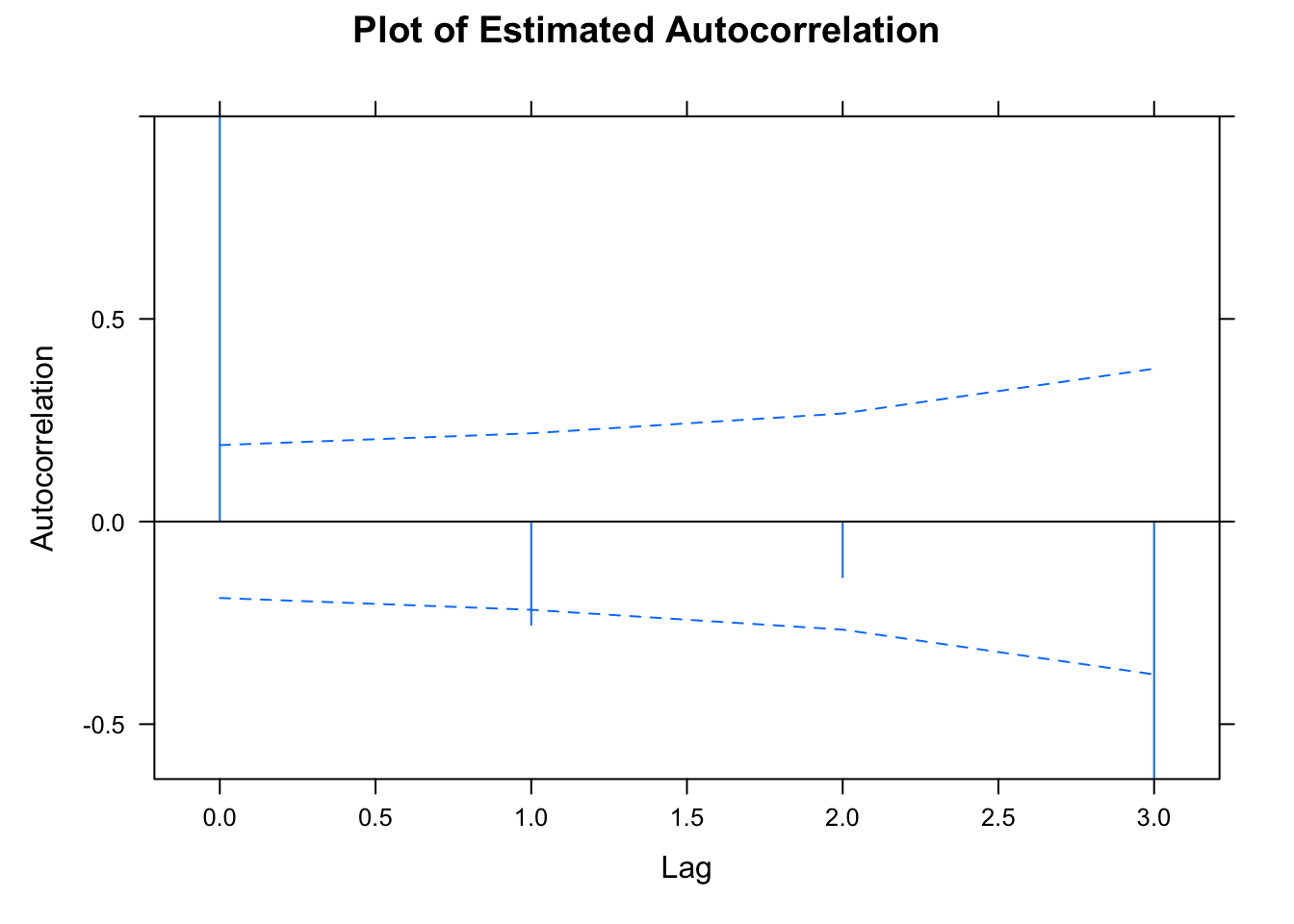
Figure 5.5: ACF plot for assessing serial correlation in the fitted model.

plot(Variogram(fitLME_intercept, form = ~ age | subject, collapse = "none",
     restype = "pearson"), xlab = "years", main = "Variogram Plot")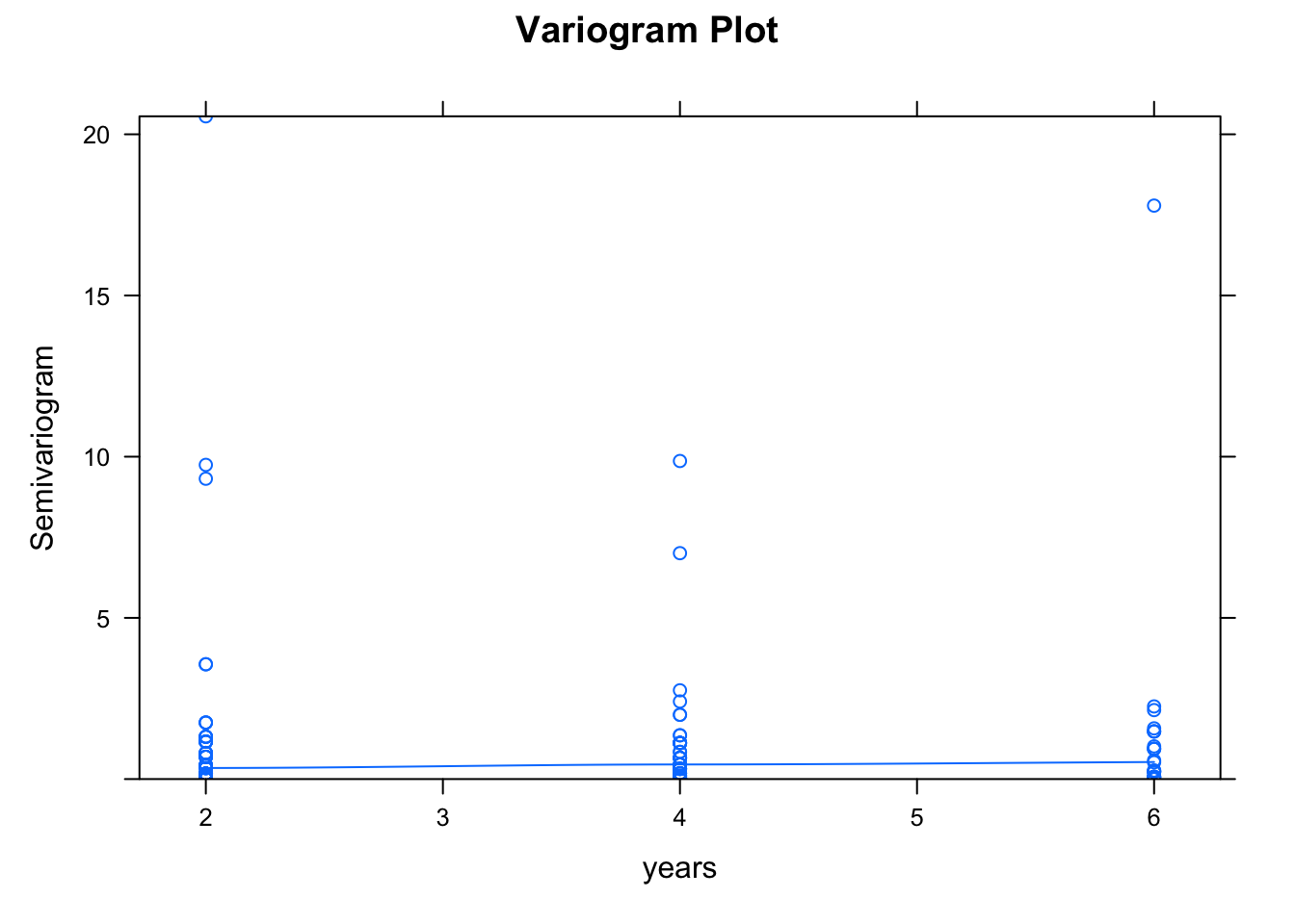

Figure 5.6: Variogram plot for assessing serial correlation in the fitted model.

In Figures 5.5 and 5.6, we have plotted the estimated autocorrelation at various lags and also plotted a 95% confidence interval for the values. Ignoring the first value (lag = 0), we do have lags at which the values fall outside of the 95% confidence interval, indicating issues with serial correlation. However, the trend line variogram does not show any obvious patterns or trends. We see it is perhaps an outlier that is driving the serial correlation to be so high. Based on the information from both of these plots together, we see that serial correlation is not evident in this model and our choice of correlation structure was adequate.

If the trend line on the variogram had not appeared to be flat, we could refit the model using other correlation structures and re-assess the fit.

Common Variances

We next assess the common variance assumption (sometimes referred to as homoscedasticity). We can do this visually by looking at a plot of the residuals.

plot(residuals(fitLME_intercept), main = "Plot of Residuals for Random Intercept Model")

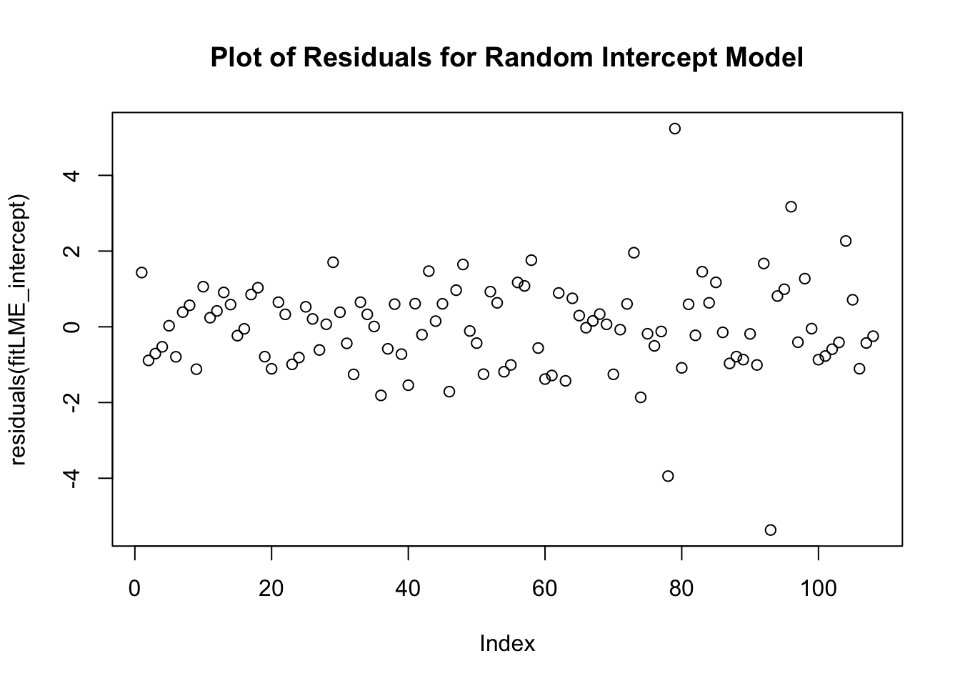
Figure 5.7: Residual plot used to assess homoscedasticity.

From Figure 5.7, we do not see any clustering or patterns, or many values outside of 2 standard deviations, indicating we have likely satisfied the common variance assumption. We can similarly look at a different plot:

plot(fitLME_intercept, subject ~ resid(.), horizontal = F, 
     panel = function(x,y){panel.bwplot(x,y)},
     main = "Boxplot of Standardized Residuals by Subject")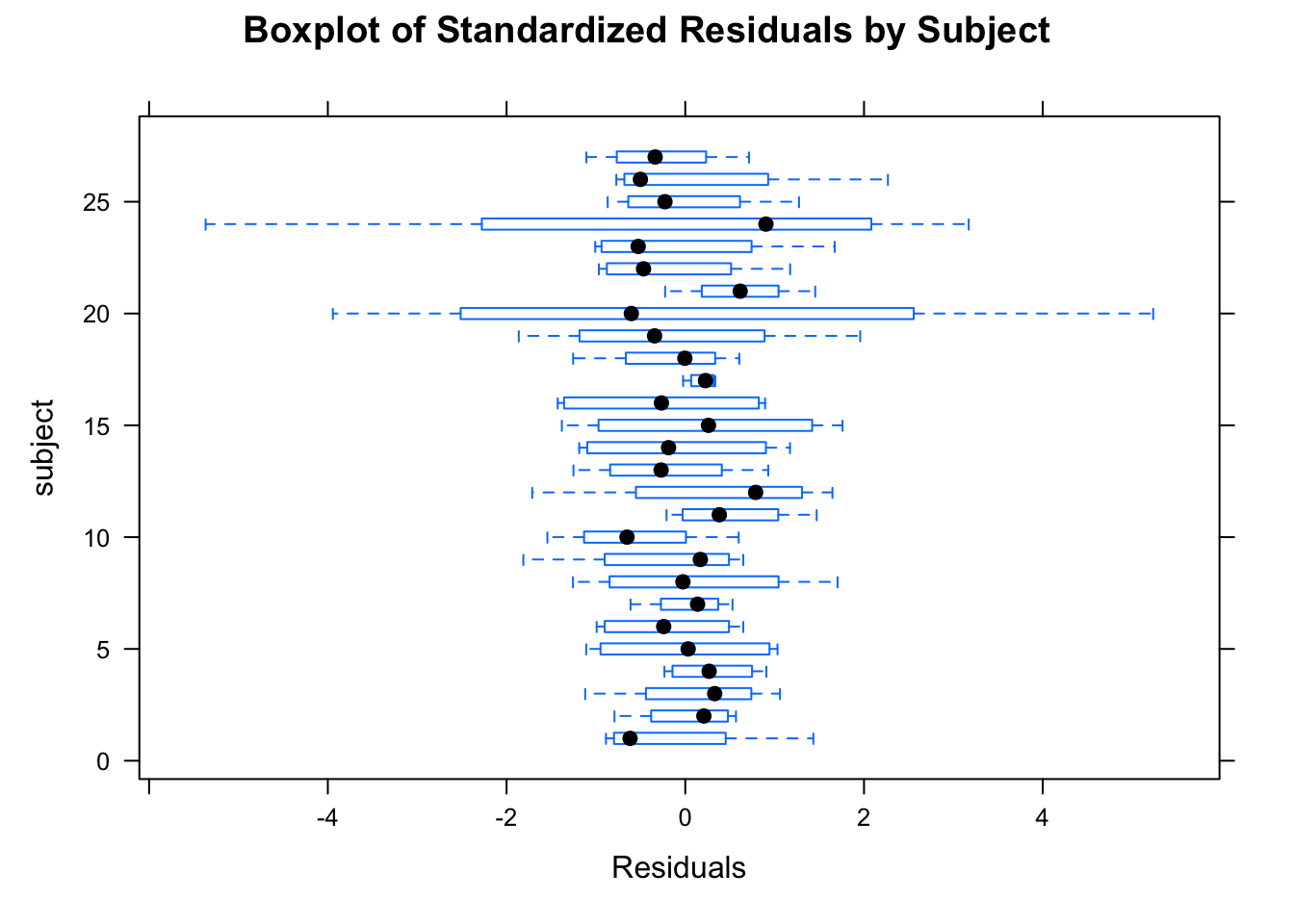

Figure 5.8: Box plot of residuals used to assess homoscedasticity.

We do not see any systematic over/under of the residuals about 0 in Figure 5.8. This indicates we have indeed satisfied the assumption.

Normality of Errors

The next assumption we can check is the normality assumption for the random error term. We can check this using a Q-Q plot of the residuals:

qqnorm(fitLME_intercept, ~ resid(.), id = 0.05, abline = c(0,1), 
       main = "Q-Q Plot of Residuals")

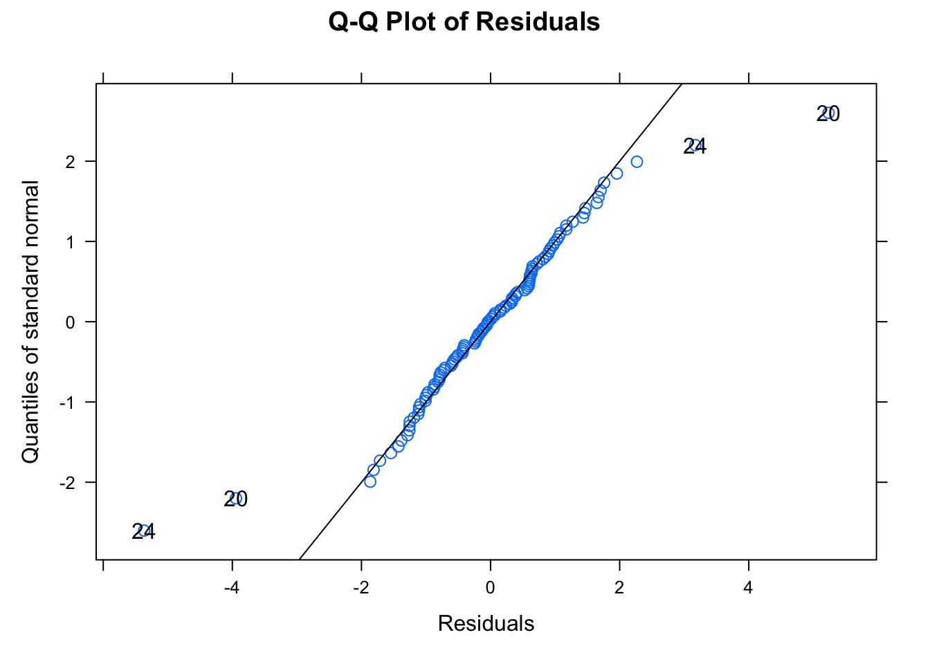
Figure 5.9: Q-Q plot for assessing normality of the random error term.

Most points lie on the line in Figure 5.9, indicating that the normality assumption is satisfied for the residuals.

We can also check the assumption of normality for the random intercepts in our model by performing the following:

qqnorm(fitLME_intercept, ~ranef(.), id = 0.05, abline = c(0,1),
       main = "Q-Q plot of Predicted Random Intercepts")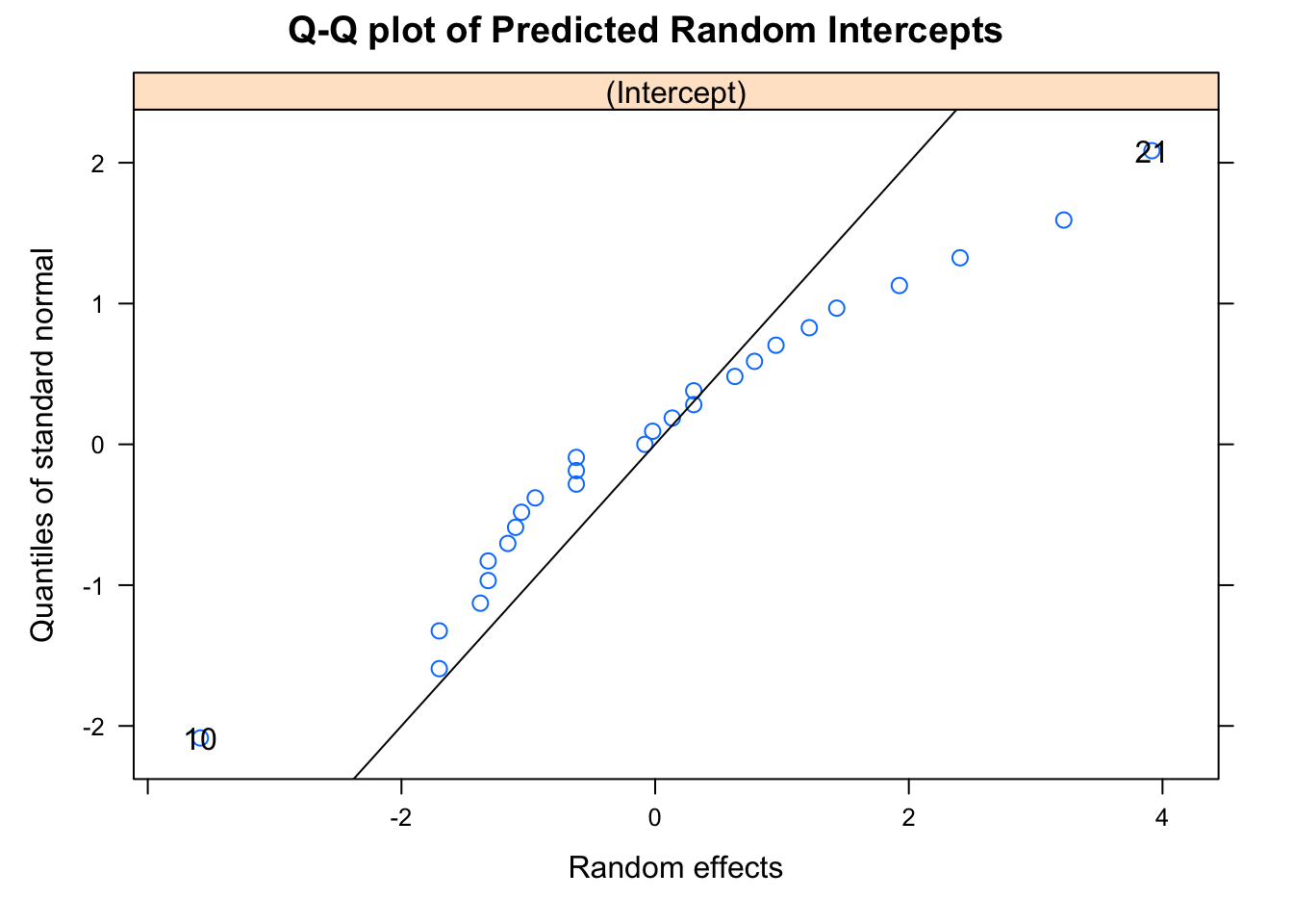

Figure 5.10: Q-Q plot for assessing normality assumption for the random intercepts.

In Figure 5.10, the Q-Q plot indicates that we do not have exactly normally distributed random intercepts. However, we often see in practice that the predicted random effects do not perfectly satisfy the normality assumption. In this setting, we consider this to be adequate for our assumption.

Linearity

The next assumption we check is the linearity assumption. We can first check this for the entire study population:

plot(fitLME_intercept, distance ~ fitted(.), id = 0.05, abline = c(0,1),
     main = "Observed vs. Fitted Values")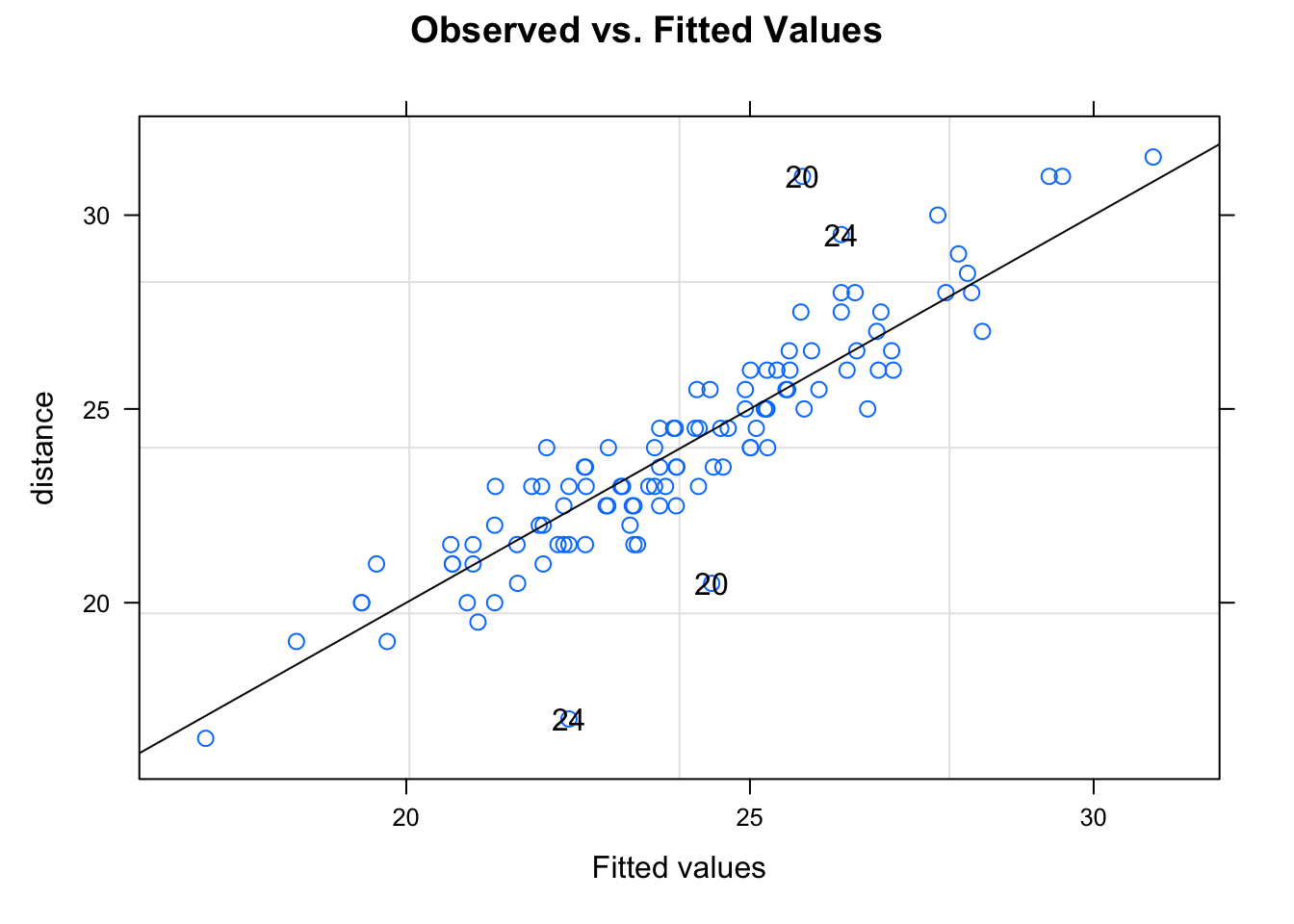

Figure 5.11: Plot for assessing linearity.

Linearity appears to be satisfied here. We can also look at linearity within each treatment group:

plot(fitLME_intercept, distance ~ fitted(.)|sex, id = 0.05, abline = c(0,1),
     main = "Observed vs. Fitted Values by Treatment Group")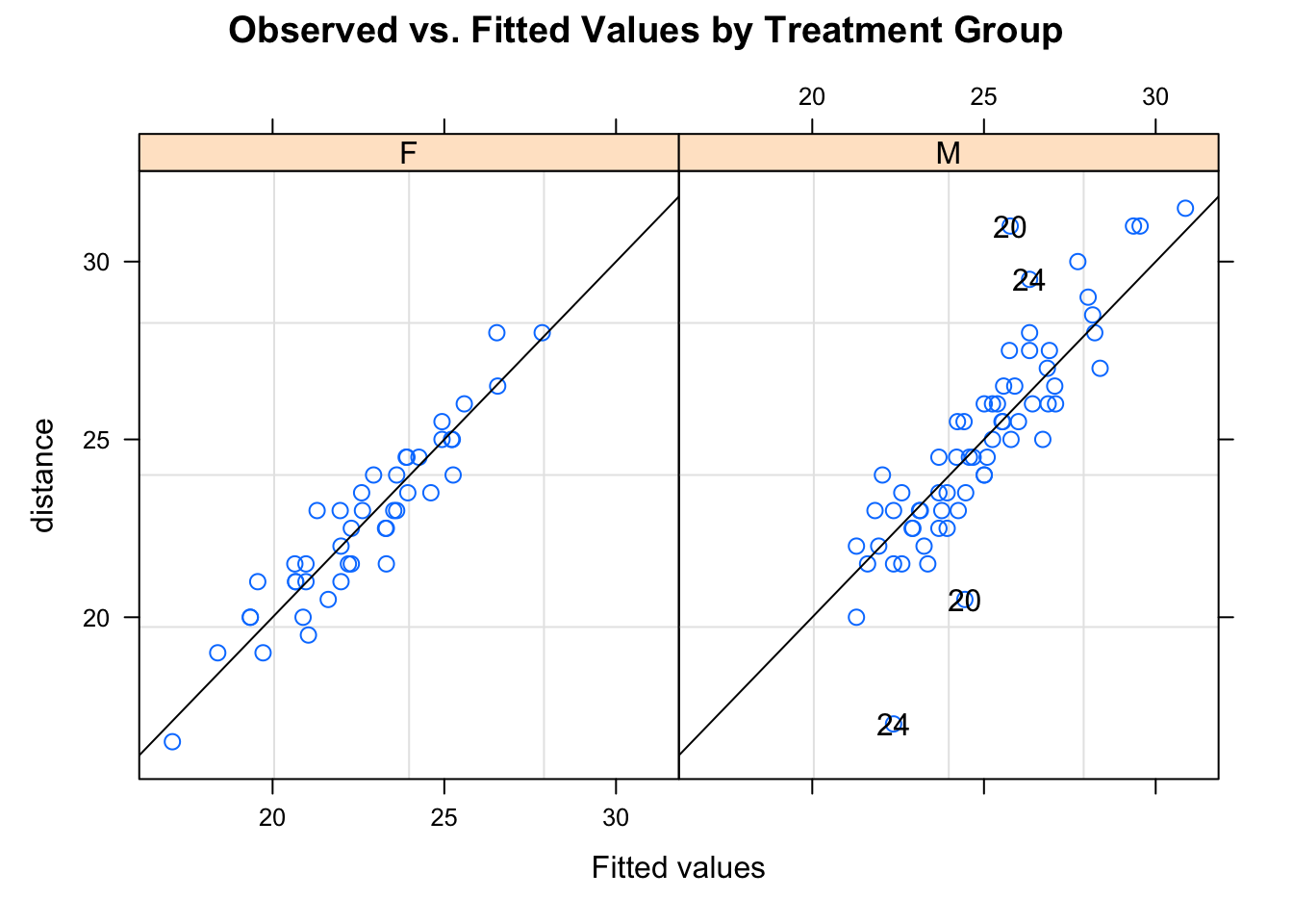

Figure 5.12: Plot for assessing linearity within each treatment group.

The assumption of linearity again appears to be satisfied. Finally, we can check for linearity in each of the 27 subjects:

plot(fitLME_intercept, distance ~ fitted(.)|subject, id = 0.05, abline = c(0,1),
     main = "Observed vs. Fitted Values by Treatment Group")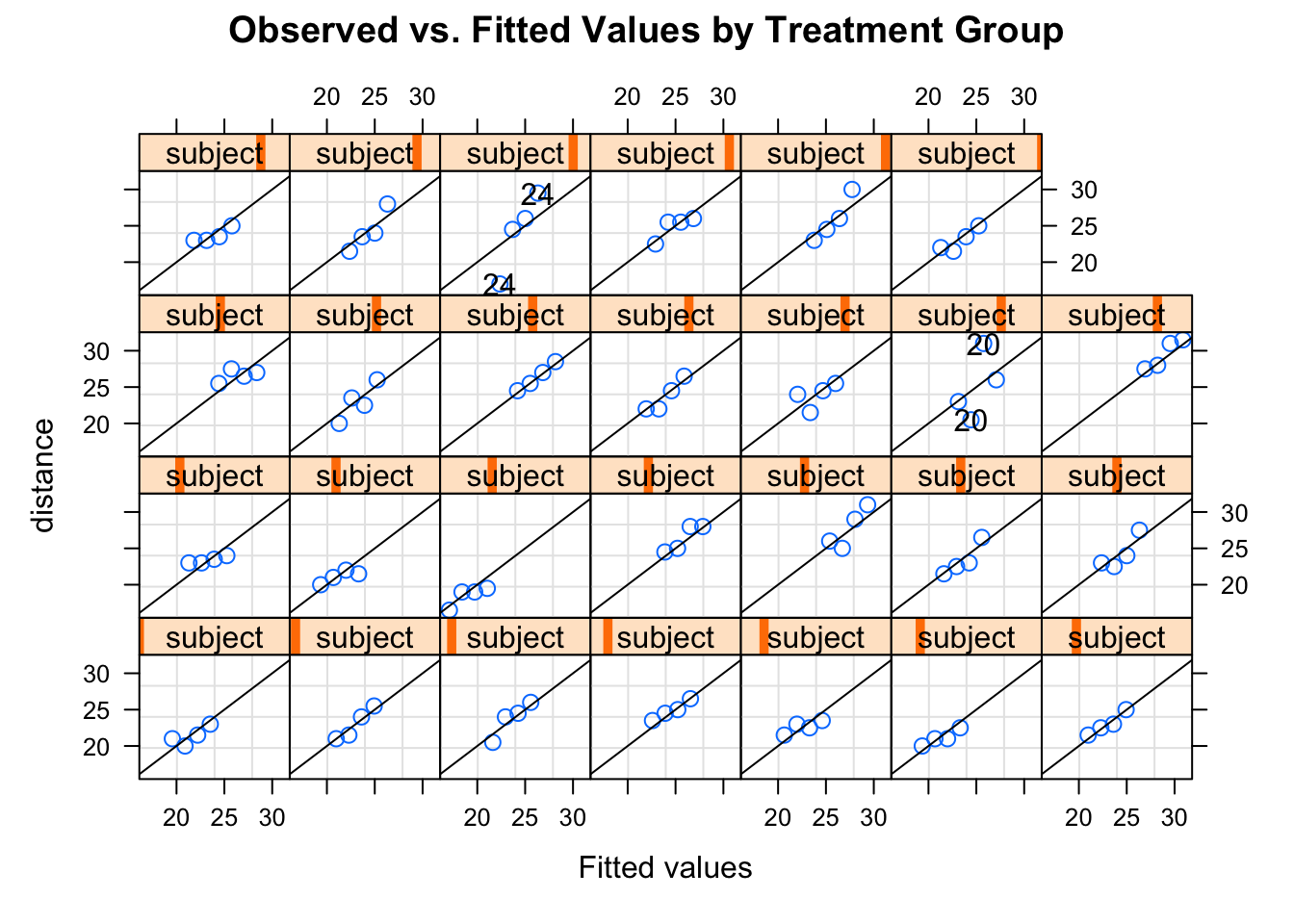

Figure 5.13: Plot for assessing linearity for each subject.

We have a small number of observations per subject, but linearity also appears to be satisfied in this settings.

5.4.7 Population Means

Finding the estimates and 95% confidence intervals for fixed and random effects is straightforward in R. We can call the intervals() function on the model of interest, as:

intervals(fitLME_intercept)

## Approximate 95% confidence intervals
## 
##  Fixed effects:
##                  lower       est.      upper
## (Intercept) 13.6026236 15.3856902 17.1687569
## age          0.5375855  0.6601852  0.7827849
## sexM         0.7528554  2.3210227  3.8891901
## attr(,"label")
## [1] "Fixed effects:"
## 
##  Random Effects:
##   Level: subject 
##                    lower     est.    upper
## sd((Intercept)) 1.310394 1.807425 2.492978
## 
##  Within-group standard error:
##    lower     est.    upper 
## 1.226126 1.431592 1.671489

From this output, we can make inferences. For example, we see that the an increase of one year in age corresponds to an estimated increase in the distance of 0.6602 (95% CI: 0.5376, 0.7823), controlling for sex.

We can also gain insights on the variability in the data. For example, we have an estimated standard error of the random intercept of 1.807 and an estimated within-group standard error of 1.4312. this tells us that we have stronger between subject variability in this model.

We can also use this model to make predictions. For example, we can predict the distance of a 13 year old male. We first create a data set for this hypothetical individual, assigning it an id of 100, and then predict:

# create the new subject
newdat <- data.frame(subject = 100, sex = 1, age = 13)

# predict (level = c(0) provides individual subject prediction)
predict(fitLME_intercept, newdata = newdat, level = c(0))[1]

## [1] 26.28912

We estimate the distance for a 13 year old male to be 26.2891.

5.4.8 Hypothesis Testing for Fixed Effects

We may be interested in performing hypothesis tests on the fixed effects’ parameters (\(\bm{\beta}\)) of the linear mixed effects model. For tests on single parameters, we can employ the summary() function to perform a t-test.

summary(fitLME_intercept)

## Linear mixed-effects model fit by REML
##   Data: dental_long 
##        AIC      BIC    logLik
##   447.5125 460.7823 -218.7563
## 
## Random effects:
##  Formula: ~1 | subject
##         (Intercept) Residual
## StdDev:    1.807425 1.431592
## 
## Fixed effects:  distance ~ age + sex 
##                 Value Std.Error DF   t-value p-value
## (Intercept) 15.385690 0.8959848 80 17.171820  0.0000
## age          0.660185 0.0616059 80 10.716263  0.0000
## sexM         2.321023 0.7614168 25  3.048294  0.0054
##  Correlation: 
##      (Intr) age   
## age  -0.756       
## sexM -0.504  0.000
## 
## Standardized Within-Group Residuals:
##         Min          Q1         Med          Q3         Max 
## -3.74889609 -0.55034466 -0.02516628  0.45341781  3.65746539 
## 
## Number of Observations: 108
## Number of Groups: 27

The output provides us with the test statistic (\(t\)-value) and associated \(p\)-value for the test of \(H_0: \beta_j = 0\) for each coefficient. For example, for the test of if age is significantly associated with distance in our dental data set, we may be interested in the test \(H_0: \beta_1 = 0\). From the output, we see the test statistic is 10.716 and the \(p\)-value is 0.0000, meaning we reject the null hypothesis and conclude that age is associated with distance, while controlling for sex.

We can perform more general hypothesis tests of the for \(H_0: \bm{C}\bm{\beta} = 0\) vs \(H_a: \bm{C}\bm{\beta} \ne 0\) using the following function:

waldTestFunction <- function(C, lme){
  # outputs results of Wald test on fixed effects for H_0: C*beta = 0 
  #
  # C: matrix for the hypothesis test H_0: C*Beta = 0
  # lme: lme object (fitted model)
  
  if(is.vector(C)){
    invisible(C = matrix(C, nrow = 1))
  }
  
  wald_stat = (t(as.matrix(lme$coefficients$fixed)) %*% t(C)) %*% 
    solve(C %*% as.matrix(lme$varFix) %*% t(C)) %*% 
    (C %*% as.matrix(lme$coefficients$fixed))
  
  df = min(dim(C)[1], dim(C)[2])
  
  p_value <- 1 - pchisq(wald_stat, df)
  
  if(p_value >= 0.001){
    cat('\n', 'Wald test chi-squared statistic is', round(wald_stat, 4), 'with', df, 'df, p-value =', round(p_value, 4), '.', '\n')
  } else {
    cat('\n', 'Wald test chi-squared statistic is', round(wald_stat, 4), 'with', df, 'df, p-value <0.001.', '\n')
  }
}

Hypotheses such as testing if the effect is the same over more than two treatments (for example, \(H_0: \beta_1 = \beta_2 = \beta_3 = 0\) in a hypothetical model) can be tested using this function.

5.4.9 Model Fitting Procedure

We summarize the model fitting procedure in the following steps:

1. read in and clean the data, and then

2. check assumptions (see Section 5.3.1). We note that we do not require observation times to be the same for individuals in this model, as this model can account for unbalanced data.

If the normality assumption is satisfied, we may start with the model fitting procedure. We then

3. focus on the time trend of response, ignoring any covariates other than those highly important such as treatment classifications. Assess whether we should have continuous or discrete time variables, higher-order terms, interactions), then

4. determine the appropriate random effects structures (do we need random intercepts, slopes?), then

5. perform variable selection on time-dependent and time-invariant covariates (including looking at interactions, non-linear terms), and finally

6. assess model diagnostics, and iterate through above steps (if needed) until a final model is selected for the research question of interest.

Once an adequate model is found, we can interpret the model and answer the research question(s).

We note that the model building process can be done with the consultation of expert opinions, if available, to include “a priori” variables in the model that should be included regardless of statistical significance.

5.4.10 Example - Milk Protein and Diet

We follow the model fitting procedure presented in 5.4.9 to answer a different research question on a new data set. We will be using the Milk data set from the nlme package. In this data set, 79 cows on different diets had measurements taken of the protein content of their milk on a weekly basis. In this data set, some measurements were missed causing an unbalanced data set. We will examine whether there was a difference in milk protein content between diets, and whether or not protein content varied over time.

Step 1: Data Read in and Cleaning

We first read in our data set using the following R commands:

data(Milk)
head(Milk)

## Grouped Data: protein ~ Time | Cow
##   protein Time Cow   Diet
## 1    3.63    1 B01 barley
## 2    3.57    2 B01 barley
## 3    3.47    3 B01 barley
## 4    3.65    4 B01 barley
## 5    3.89    5 B01 barley
## 6    3.73    6 B01 barley

We see that our data is already in long form where we have one row per observation, and multiple rows for each subject, so we do not need to further process the data.

Step 2: Assessing Normality

We can begin to explore the data. We first need to assess the normality of the outcome of interest, protein. We can do this by looking at the distribution of the outcome by generating a histogram and also a Q-Q plot.

# set graphs to appear in one row and 2 columns (side by side)
par(mfrow = c(1,2)) 

# histogram of the outcome
hist(Milk$protein, xlab = "Protein Content", main = "Histogram of Outcome")

# Q-Q plot and line
qqnorm(Milk$protein) # plots quantiles against std normal distribution
qqline(Milk$protein)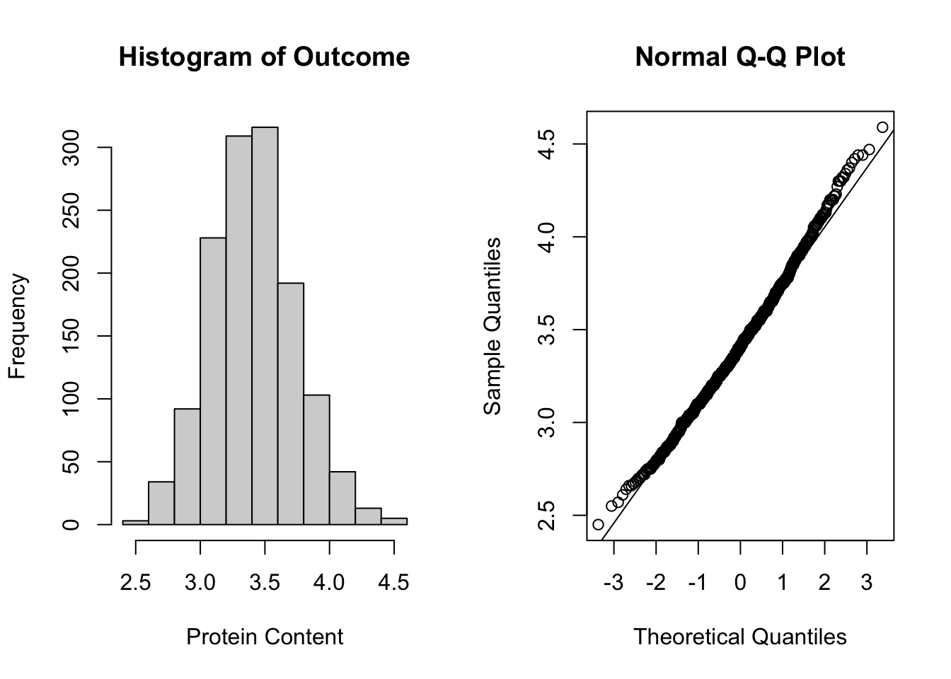

Figure 5.14: Plots used to assess normality.

From these plots in Figure 5.14, it appears that we have satisfied the normality assumption.

Step 3: Assessing Time Trend

The next step in our analysis is to assess the time trend. We first visualize the individual cow’s protein content over time using a spaghetti plot.

ggplot(data = Milk, aes(x = Time, y = protein, group = Cow)) +
  geom_line() +
  facet_grid(. ~ Diet) +
  ggtitle("Spaghetti Plot for Cow Protein Content (Stratified by Diet)")

Figure 5.15: Spaghetti plot of individual cows, stratifiet by diet group.

Due to the large number of subjects in the data set, it is quite difficult to look at the time trends and see patterns within each group from the individual. We note that for data with irregular observation timings, it is not appropriate to look at the mean protein level at each observation (as we did in previous examples with balanced longitudinal data). As such, we can use a technique to visualize the time trend by looking at a smoothed estimate of the average time trend within each diet group using LOESS.

To do so, we can plot the following:

ggplot(data = Milk, aes(x = Time, y = protein)) + 
  geom_smooth() + # plots smoothed estimate
  facet_grid(. ~ Diet) + # groups by diet group
  ggtitle("LOESS Curves of Protein Content by Diet Group") # adds title

Figure 5.16: LOESS curves used to assess time trend by group.

On average, we see non-linear time trends and different trends by group, particularly for the lupins only diet group. We thus want to consider including higher order time variables to account for the non-linear trend, and also consider interactions to allow for the time trend to differ by diet group. With a large number of observations per subject, we treat Time (in weeks) as a continuous time variable.

When assessing the form of the time trend, we include integral variables like the treatment assignment (in our case, diet) and assume an unstructured correlation structure in our model. From the spaghetti plot in Figure 5.15, we see cows have varying baseline measurements (intercepts) and time trends (slopes) and thus we should consider starting with a random intercept and slope model. As such, we start with the following model:

\[ \mu_{ij} = \beta_0 + \beta_1D1_{i} + \beta_2D2_i + \beta_3t_{ij} + b_{0,i} + b_{1, i} \] where \(D1_i = 1\) if cow \(i\) is on diet 1 (barley only), \(D2_i = 1\) if cow \(i\) is on diet 2 (barley + lupins), \(t_{ij}\) is the time since calving (in weeks), \(b_{0,i}\) is the random intercept that allows cows to have varying baseline protein content measurements, and \(b_{1,i}\) is the random slope that allows the time trend to vary by cow. Note we are comparing diets to the lupins only diet (reference diet).

We fit this model with an unstructured correlation structure to begin using the ML method (as we are interested in fixed effects right now), using the following code:

# first make variables for diet groups
Milk$D1 <- ifelse(Milk$Diet == "barley", 1, 0)
Milk$D2 <- ifelse(Milk$Diet == "barley+lupins", 1, 0)
Milk$D3 <- ifelse(Milk$Diet == "lupins", 1, 0)


fitcows1 <- lme(
  fixed = protein ~ D1 + D2 + Time, # specify fixed effects
  random = ~ Time| Cow, # random slope on time variable,
  # Intercept is included by default
  data = Milk,
  method = "ML"
) # default unstructured correlation for
# random effects and independence for within-subj correlation

We wish to compare this model to one including higher-order time terms. We create a squared time term as a fixed effect and fit an additional model as:

# First create a squared time term
Milk$Timesq <- (Milk$Time)^2

# fit model including new time^2 variable as a fixed effect
fitcows2 <- lme(
  fixed = protein ~ D1 + D2 + Time + Timesq, # specify fixed effects
  random = ~ Time| Cow, # random slope on time variable,
  # Intercept is included by default
  data = Milk,
  method = "ML"
) # default unstructured correlation for
# random effects and independence for within-subj correlation

We then can see which model fit is better using an LRT. The null hypothesis is that the simpler model (fitcows1) fits as well as the more complex model (fitcows2). We do this in R by:

anova(fitcows1, fitcows2)

##          Model df      AIC      BIC    logLik   Test  L.Ratio p-value
## fitcows1     1  8 358.1166 399.7021 -171.0583                        
## fitcows2     2  9 309.1581 355.9418 -145.5791 1 vs 2 50.95847  <.0001

We reject the null hypothesis and conclude that the more complex model provides a better fit due to the small \(p\)-value. As such, we continue looking at our time trend from this model. We may want to consider cubic time terms. As such, we fit a model including Time^3 as a covariate, and perform another LRT.

# First create a squared time term
Milk$Timecb <- (Milk$Time)^3

# fit model including new time^2 variable as a fixed effect
fitcows3 <- lme(
  fixed = protein ~ D1 + D2 + Time + Timesq + Timecb, # specify fixed effects
  random = ~ Time| Cow, # random slope on time variable,
  # Intercept is included by default
  data = Milk,
  method = "ML"
) # default unstructured correlation for
# random effects and independence for within-subj correlation

# Perform LRT of model including cubic time term vs not
anova(fitcows2, fitcows3)

##          Model df      AIC      BIC     logLik   Test  L.Ratio p-value
## fitcows2     1  9 309.1581 355.9418 -145.57906                        
## fitcows3     2 10 192.8049 244.7868  -86.40246 1 vs 2 118.3532  <.0001

The small \(p\)-value tells us that we should in fact include the cubic time term in our model. We continue model building from fitcows3.

The next step is to see if we need to include interaction terms for the diet groups. We first consider interactions on the linear time term. We create this variable in R and then fit the model and perform another LRT:

# Create the interaction of the diet and linear time term
Milk$inter_D1Time <- Milk$Time*Milk$D1
Milk$inter_D2Time <- Milk$Time*Milk$D2

# Fit model including this interaction
fitcows4 <- lme(
  fixed = protein ~ D1 + D2 + Time + Timesq + Timecb +
    inter_D1Time + inter_D2Time, # specify fixed effects
  random = ~ Time| Cow, # random slope on time variable,
  # Intercept is included by default
  data = Milk,
  method = "ML"
) # default unstructured correlation for
# random effects and independence for within-subj correlation

# Perform LRT of model including linear interaction vs not
anova(fitcows3, fitcows4)

##          Model df      AIC      BIC    logLik   Test  L.Ratio p-value
## fitcows3     1 10 192.8049 244.7868 -86.40246                        
## fitcows4     2 12 195.2882 257.6664 -85.64411 1 vs 2 1.516694  0.4684

We fail to reject the null hypothesis with this large \(p\)-value, and conclude that we can use the model without linear interactions. We continue with fitcows3 for our analysis.

Step 4: Consider Appropriate Random Effects Structure

Now that the time trend has been assessed, we can focus on choosing the random effects. In the previous model, we assumed that we had a random intercept and a random slope on the linear time covariate. We can first investigate whether or not the random slope was needed by comparing the model to one that does not include a random slope for time.

We first need to fit/refit these models in R using the REML method (default) as we are interested in inference on the random effects structure and then perform an LRT (with caution that we cannot use the given \(p\)-value). The degrees of freedom is 1 because the models differ by one random effect.

# refit model using REML

fitcows3_REML <- lme(
  fixed = protein ~ D1 + D2 + Time + Timesq + Timecb, # specify fixed effects
  random = ~ Time| Cow, # random slope on time variable,
  # Intercept is included by default
  data = Milk,
  method = "REML"
) # default unstructured correlation for
# random effects and independence for within-subj correlation



# fit model without random slope on time

fitcows5_REML <- lme(
  fixed = protein ~ D1 + D2 + Time + Timesq + Timecb, # specify fixed effects
  random = ~ 1 | Cow, # random intercept only
  # Intercept is included by default
  data = Milk,
  method = "REML"
) # default unstructured correlation for
# random effects and independence for within-subj correlation

# perform LRT but ignore the p-value
LRT_mix_cows35 <- anova(fitcows3_REML, fitcows5_REML)
teststat_mix_cows35 <- LRT_mix_cows35$L.Ratio[2]
pchibarsq(teststat_mix_cows35, df = 1, mix = 0.5) # degree of freedom is 1

## [1] 1

The \(p\)-value is large, indicating that we do not have evidence to reject the null hypothesis that the simpler model is better. As such, we can continue analysis without the random effect on the linear time term (fitcows5). We can still check whether we should have a random effect on higher-order time trends by comparing the intercept only model (fitcows5) to a new model including random effects on timesq and timecb:

# fit model without random slope on timesq and timecb

fitcows6_REML <- lme(
  fixed = protein ~ D1 + D2 + Time + Timesq + Timecb, # specify fixed effects
  random = ~  Timesq + Timecb | Cow, # random int and slopes
  # Intercept is included by default
  data = Milk,
  method = "REML"
) # default unstructured correlation for
# random effects and independence for within-subj correlation

# perform LRT but ignore the p-value
LRT_mix_cows56 <- anova(fitcows5_REML, fitcows6_REML)
teststat_mix_cows56 <- LRT_mix_cows56$L.Ratio[2]
pchibarsq(teststat_mix_cows56, df = 1, mix = 0.5) # degree of freedom is 1

## [1] 1

It is unsurprising that we also fail to reject this null hypothesis. We confirm that we should continue analysis with the random intercept only model (fitcows5).

Step 5: Variable Selection Using our current model, fitcows5, we consider other fixed effect variables at our disposal. If we had more variables to add into our model, we could add them and fit the model using the ML method and perform a LRT to see if the model fit is better with those variables included.

Although we do not have more variables to consider at our data set, we can still look at our current model and see if all variables we included at the beginning are necessary. We first must re-fit the model using the ML method as we are interested again with the fixed effects.

# fit model without random slope on time
fitcows5<- lme(
  fixed = protein ~ D1 + D2 + Time + Timesq + Timecb, # specify fixed effects
  random = ~ 1 | Cow, # random intercept only
  # Intercept is included by default
  data = Milk,
  method = "ML"
) # default unstructured correlation for
# random effects and independence for within-subj correlation

summary(fitcows5)

## Linear mixed-effects model fit by maximum likelihood
##   Data: Milk 
##        AIC      BIC    logLik
##   327.5777 369.1632 -155.7889
## 
## Random effects:
##  Formula: ~1 | Cow
##         (Intercept)  Residual
## StdDev:   0.1651774 0.2556705
## 
## Fixed effects:  protein ~ D1 + D2 + Time + Timesq + Timecb 
##                 Value  Std.Error   DF   t-value p-value
## (Intercept)  3.766946 0.04714803 1255  79.89615  0.0000
## D1           0.204011 0.04915651   76   4.15023  0.0001
## D2           0.108376 0.04820020   76   2.24847  0.0274
## Time        -0.173380 0.01442092 1255 -12.02284  0.0000
## Timesq       0.016945 0.00169194 1255  10.01533  0.0000
## Timecb      -0.000480 0.00005705 1255  -8.41528  0.0000
##  Correlation: 
##        (Intr) D1     D2     Time   Timesq
## D1     -0.501                            
## D2     -0.511  0.491                     
## Time   -0.641 -0.001 -0.002              
## Timesq  0.572  0.001  0.002 -0.974       
## Timecb -0.518 -0.002 -0.002  0.926 -0.986
## 
## Standardized Within-Group Residuals:
##         Min          Q1         Med          Q3         Max 
## -3.06241162 -0.65172129  0.05634077  0.65653761  3.65613145 
## 
## Number of Observations: 1337
## Number of Groups: 79

This model can be written as:

\[ \mu_{ij} = \beta_0 + \beta_1D1_{i} + \beta_2D2_i + \beta_3t_{ij} + \beta_4t_{ij}^2 + \beta_5t_{ij}^3 + b_{0,i} \]

Looking at the summary of this model, it appears that most covariates are statistically significant. We can still do a test to see if the treatment variables are necessary in the model. To do so, we perform a hypothesis test of \(H_0: \beta_1 = \beta_2 = 0\). To do so, we employ the waldTestFunction presented in 5.4.8. To perform this test, we need to create a matrix \(\bm{C}\) that will indicate the hypothesis test we wish to perform. \(\bm{C}\) will have one column for each coefficient for fixed effects (including \(\beta_0\)), and one row for each coefficient in our hypothesis test. In this case, we let

\[ \bm{C} = \begin{bmatrix} 0 & 1 & 0 & 0 & 0 & 0 \\ 0 & 0 & 1 & 0 & 0 & 0 \\ \end{bmatrix} \] and perform the hypothesis test in R by:

Cmat <- rbind(c(0,1,0,0,0,0),
              c(0,0,1,0,0,0))

waldTestFunction(Cmat, fitcows5)

## 
##  Wald test chi-squared statistic is 17.3612 with 2 df, p-value <0.001.

We reject the null hypothesis and conclude that at least one of \(\beta_1\) or \(\beta_2\) is not zero.

Although we had already assessed the form of the time trend, we should double check that the form is still appropriate as our random effects structure has changed (we assessed the time trend assuming a random slope on time, which we since removed). For the hypothesis test seeing if we need the cubic time term, we can look at the model summary. The \(p\)-value for \(\beta_5 = 0\) is 0.0000, indicating that we do need the cubic time trend. All individual time trend terms are significant, but we can still perform a hypothesis test confirming that we need all three terms, as \(H_0: \beta_3 = \beta_4 = \beta_5 = 0\). To do so, we perform the following:

Cmat2 <- rbind(c(0,0,0,1,0,0),
              c(0,0,0,0,1,0),
              c(0,0,0,0,0,1))

waldTestFunction(Cmat2, fitcows5)

## 
##  Wald test chi-squared statistic is 200.4164 with 3 df, p-value <0.001.

We reject the null hypothesis and conclude at least one of the terms is non-zero, and thus keep all three terms in the model.

Note: for individual covariates, we could look at the \(p\)-value given in the model summary for the hypothesis test of \(H_0: \beta_j = 0\) or do an LRT for nested models.

Step 6: Model Diagnostics

Now that we have fit a model, we need to perform model diagnostics to assess the fit. If the fit appears to be inadequate, we can iterate through the above procedure again until the fit is adequate. More details on diagnostics can be found in Section 5.4.6.

First we assess if there is evidence of serial correlation among the random error term in our model. We can do this by plotting a variogram:

plot(Variogram(fitcows5, form = ~ Time | Cow, collapse = "none",
     restype = "pearson", smooth = TRUE), xlab = "Weeks", main = "Variogram Plot")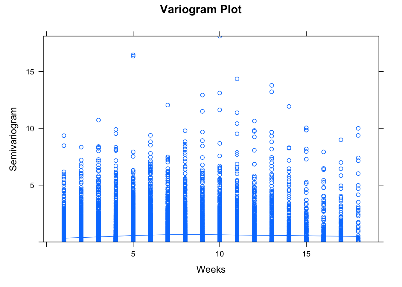

Figure 5.17: Plots used to assess serial correlation.

We do not see a systematic trend in the trend line included in the Variogram plot in 5.17. As such, we do not have evidence of serial correlation.

Next, we check the common variance assumption with

plot(residuals(fitcows5, type = "normalized"), main = "Plot of Residuals for Random Intercept Model")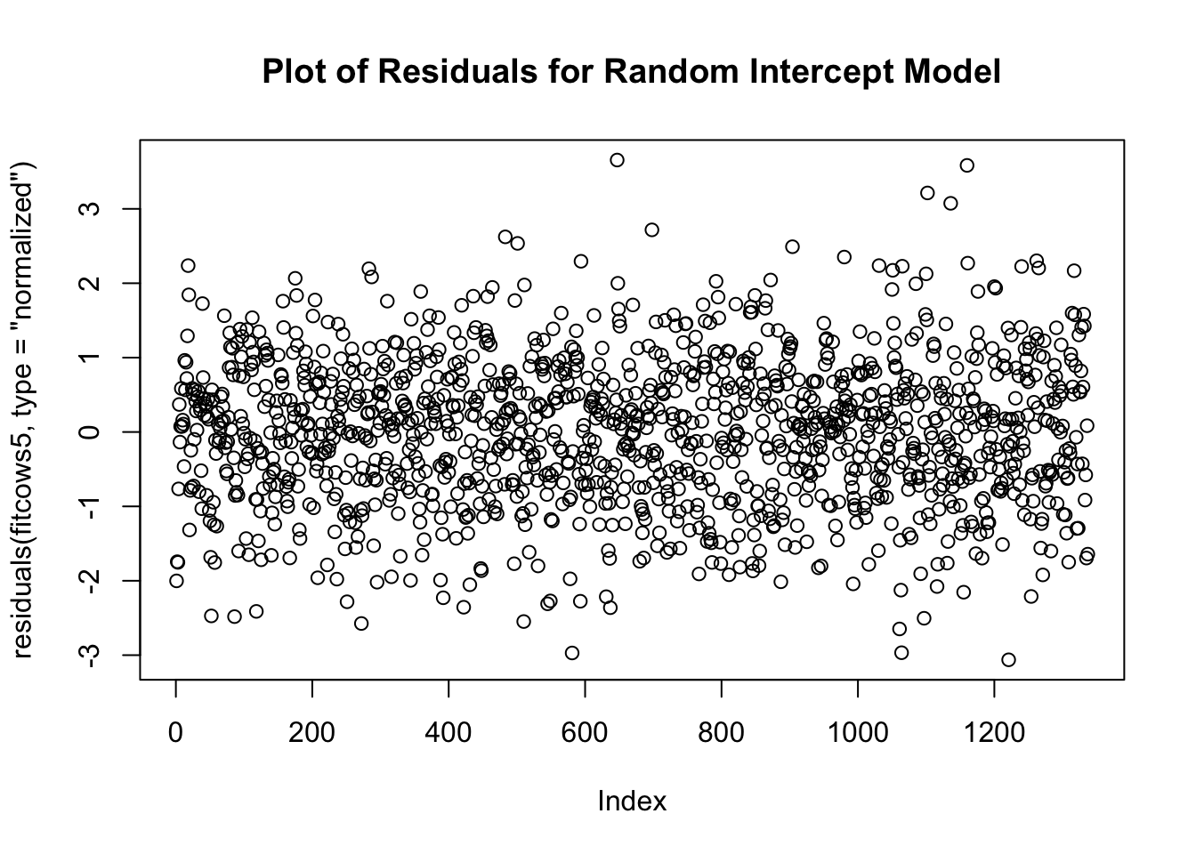

Figure 5.18: Plot for assessing common variance assumption.

The residuals appear to be randomly spread out about 0 with most observations within 2 standard deviations, with the exception of a few outliers.

We next check the normality of errors assumption. We do this by creating a Q-Q plot of the residuals:

qqnorm(fitcows5, 
       main = "Q-Q Plot of Residuals", abline = c(0,1))

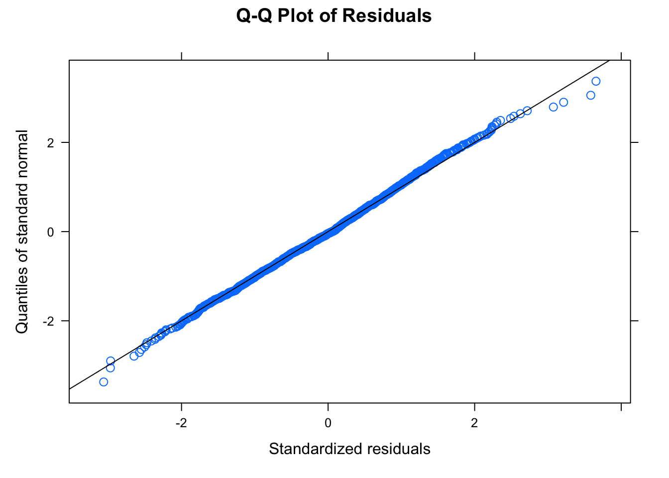
Figure 5.19: Plor for assessing normality of random error term.

From the plot in Figure 5.19, we appear to satisfy the normality of errors assumption.

Next, we look at the normality of the random intercept:

qqnorm(fitcows5, ~ranef(.), id = 0.05, abline = c(0,10), # abline adjusted due to scale
       main = "Q-Q plot of Predicted Random Intercepts")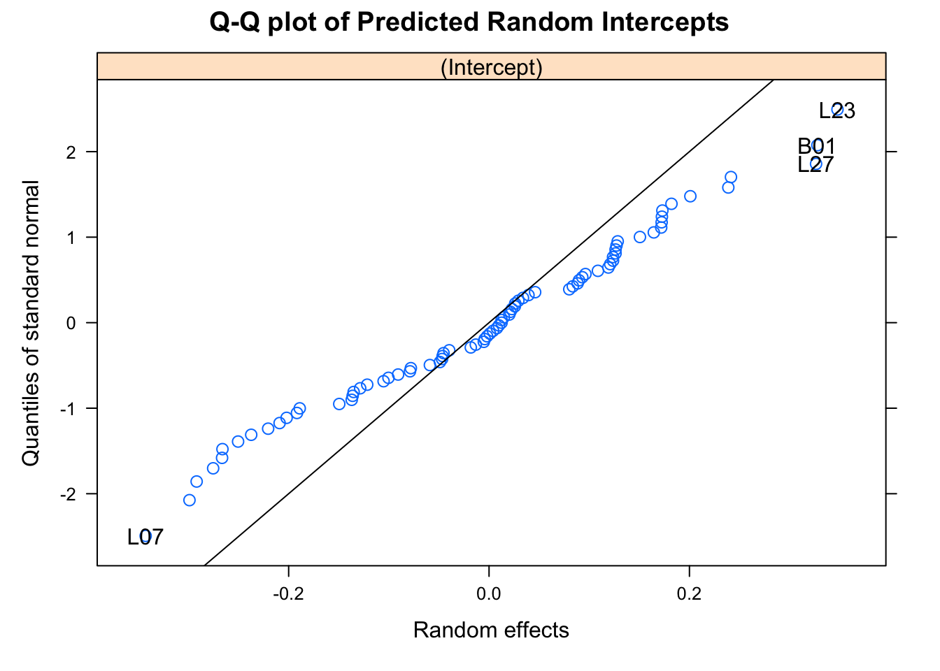

Figure 5.20: Plot for assessing normality of random intercept term.

In Figure 5.20, the Q-Q plot indicates that we do not have exactly normally distributed random intercepts. However, we often see in practice that the predicted random effects do not perfectly satisfy the normality assumption. In this setting, we consider this to be adequate for our assumption.

We next assess linearity, which we can do my looking at the observed versus fitted values over the entire study population:

plot(fitcows5, protein ~ fitted(.), abline = c(0,1),
     main = "Observed vs. Fitted Values")

Figure 5.21: Plot to assess linearity in the population.

As in 5.21, we appear to have satisfied the linearity assumption. We can also check for linearity within the diet groups:

plot(fitcows5, protein ~ fitted(.)|Diet, abline = c(0,1),
     main = "Observed vs. Fitted Values")

Figure 5.22: Plot to assess linearity in each diet group.

Linearity appears to be satisfied again.

Answering the Research Questions

We have satisfied all of the model assumptions based on our diagnostics, and can move onto interpreting the model and answering the research question of interest. Let’s look again at the model summary:

summary(fitcows5)

## Linear mixed-effects model fit by maximum likelihood
##   Data: Milk 
##        AIC      BIC    logLik
##   327.5777 369.1632 -155.7889
## 
## Random effects:
##  Formula: ~1 | Cow
##         (Intercept)  Residual
## StdDev:   0.1651774 0.2556705
## 
## Fixed effects:  protein ~ D1 + D2 + Time + Timesq + Timecb 
##                 Value  Std.Error   DF   t-value p-value
## (Intercept)  3.766946 0.04714803 1255  79.89615  0.0000
## D1           0.204011 0.04915651   76   4.15023  0.0001
## D2           0.108376 0.04820020   76   2.24847  0.0274
## Time        -0.173380 0.01442092 1255 -12.02284  0.0000
## Timesq       0.016945 0.00169194 1255  10.01533  0.0000
## Timecb      -0.000480 0.00005705 1255  -8.41528  0.0000
##  Correlation: 
##        (Intr) D1     D2     Time   Timesq
## D1     -0.501                            
## D2     -0.511  0.491                     
## Time   -0.641 -0.001 -0.002              
## Timesq  0.572  0.001  0.002 -0.974       
## Timecb -0.518 -0.002 -0.002  0.926 -0.986
## 
## Standardized Within-Group Residuals:
##         Min          Q1         Med          Q3         Max 
## -3.06241162 -0.65172129  0.05634077  0.65653761  3.65613145 
## 
## Number of Observations: 1337
## Number of Groups: 79

We conclude that protein content does vary over time, in a non-linear fashion. We also can conclude that protein content varied by the type of diet that the cow was given. A barley-only diet was associated with a 0.204 unit increase in protein content compared to a lupins-only diet (controlling for time) (\(p\) = 0.0001). A barley and lupins diet was associated with a 0.108 unit increase in protein consumption compared to a lupins-only diet (controlling for time) (\(p\) = 0.0274).

We could further test if there is a difference between the barley-only and barely and lupins diets by testing the hypothesis that \(\beta_1 = \beta_2\). We can do this in R by the following:

Cmat <- rbind(c(0,1,0,0,0,0),
              c(0,0,-1,0,0,0))

waldTestFunction(Cmat, fitcows5)

## 
##  Wald test chi-squared statistic is 17.3612 with 2 df, p-value <0.001.

We reject the null hypothesis and conclude that the barley-only and the barley and lupins diets are significantly different from each other. That is, we conclude that all three diets are significantly different from each other, where the barley-only diet is associated with the highest protein content followed by the barely and lupins diet.

5.4.11 Example - AIDS Clinical Trial Group

We follow the model fitting procedure presented in 5.4.9 to answer a different research question on a new data set. We will be using data from the AIDS Clinical Trial Group (ACTG), which can be downloaded here. In this data set, 1309 AIDS patients with advanced immune suppression were randomized to one of four daily treatment regimens. Three of the regimens (Treatments 1-3) involve a dual combination of HIV-1 transcriptase inhibitors, and the fourth involves a triple combination of HIV-1 transcriptase inhibitors.

Measures of CD4 counts were scheduled to be taken at every 8 week interval during follow-up, however the data set is considered unbalanced due to mistimed measurements, skipped visits, and drop-out. Lower CD4 counts represent lower immune function.

Researchers are interested in seeing if the change in log-transformed CD4 counts (log(CD4 counts + 1)) from baseline varied between treatment groups, with increased interest in the effect of the dual vs triple combination treatments. Such transformation on the CD4 counts was proposed by experts in the field and exists as a variable in the data set. We assume any missingness and drop-out is at completely at random and does not need to be accounted for in the analysis, although this may not be true in practice.

Step 1: Data Read in and Cleaning

We first read in the data, which is located in the “data” folder, and name the columns. Note: any preamble information, such as the description of the data set should be removed from the .txt file before reading into R.

# read in the data set
aidsdat <- read.table("data/ACTG.txt")

# rename the columns
colnames(aidsdat) <- c("id", "treatment", "age", "gender", "week", "logcount")

This data is already in long form, but we need to make sure that the variables for treatment and gender are treated as categorical variables. We can do this by either renaming the variables to be characters, or by using the as.factor() function. For clarity, we will rename the gender variable, where 1 is male and 0 is female. We will keep the treatment numbers as 1 - 4 but create dummy variables (we can also assign them as as.factors() but this allows us to be more flexible):

# change gender values to M, F
aidsdat$gender <- ifelse(aidsdat$gender == 1, "M", "F") # change 1 to M, 0 to F

#create individual treatment variables
aidsdat$T1 <- ifelse(aidsdat$treatment == 1, 1, 0)
aidsdat$T2 <- ifelse(aidsdat$treatment == 2, 1, 0)
aidsdat$T3 <- ifelse(aidsdat$treatment == 3, 1, 0)
aidsdat$T4 <- ifelse(aidsdat$treatment == 4, 1, 0)

Step 2: Assessing Normality

Now that our data is the correct form, we can begin to explore the data. We first assess the normality assumption for the outcome of interest logcount. We do this by looking at the distribution of the outcome, and creating a Q-Q plot.

# set graphs to appear in one row and two columns
par(mfrow = c(1,2))

# histogram of outcome
hist(aidsdat$logcount, xlab = "Log(count + 1)", main = "Histogram of Outcome")

# QQ plot and line
qqnorm(aidsdat$logcount) # plots quantiles against st normal
qqline(aidsdat$logcount)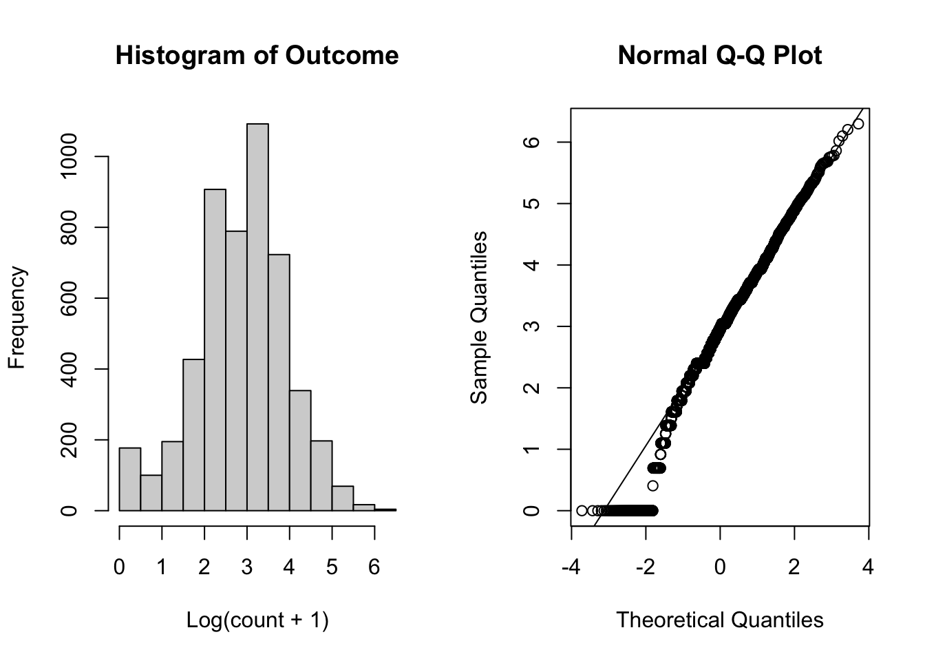

Figure 5.23: Plot for assessing normality in the ACTG data set.

From the plots in Figure 5.23, we do not have strong evidence that the normality assumption is violated as most observations are close to the theoretical quantiles in the Q-Q plot. We do see quite a few individuals with Log(1 + CD4 count) of 0. We may want to look into these observations further to determine if we should remove these from the analysis. we note that we could consider using a Generalized Linear Mixed Effect Model (GLMM) as we do have slight skewness in the distribution of our outcome. A GLMM would allow us to assign a different distribution to the outcome and is suitable for data that is not normally distributed. However, for the purpose of this analysis we will continue with the entire data set. See Section 5.3.1 for more information on tests of normality.

Step 3: Assessing Time Trend

The next step is to assess the time trend. When looking for the proper form of the time trend, we include integral variables like the treatment and assume an unstructured correlation structure in our model. We have so many observations in our data set at irregular times that many data visualization techniques previously shown to look at the time trend will fail.

To gain some insight on the time trend, we can look at a smoothed estimate of the average time trend within each treatment group, and we can also look at a small random sample of individuals and look at their individual trajectories. We can group them by treatment group, as well.

We first look at a smoothed estimate at the population trend using LOESS.

# plot response over time for this group, grouped by treatment
ggplot(data = aidsdat, aes(x = week, y = logcount)) +
  geom_smooth() +
  facet_grid(. ~ treatment) +
  scale_color_manual() +
  ggtitle("LOESS Curves of log(CD4 counts + 1) Stratified by Treatment")

Figure 5.24: Estimated curves for log(CD4 counts + 1) estimated by LOESS within each treatment group/

We see that the trend differs greatly between groups. In particular, treatment 4 (triple therapy) differs greatly from treatments 1 - 3 (dual therapies), which are similar to one another. We may want to consider higher order time terms due to the curvature in the trend for treatment 4 in particular for our fixed-effects.

Next, we look at a random sample of 50 individuals from our data set, grouped by treatment group.

# set seed so results reproducible
set.seed(100)

# randomly select 50 ids
randomids <- sample(aidsdat$id, 50)

# make data set of just those individuals that were randomly selected
aidsdat_rand <- aidsdat[which(aidsdat$id %in% randomids),]

# plot response over time for this group, grouped by treatment
ggplot(data = aidsdat_rand, aes(x = week, y = logcount, group = id)) +
  geom_line() +
  geom_point() +
  facet_grid(. ~ treatment) +
  scale_color_manual() +
  ggtitle("Spaghetti Plot for Random Sample (n = 50) of log(CD4 counts + 1) \n Stratified by Treatment")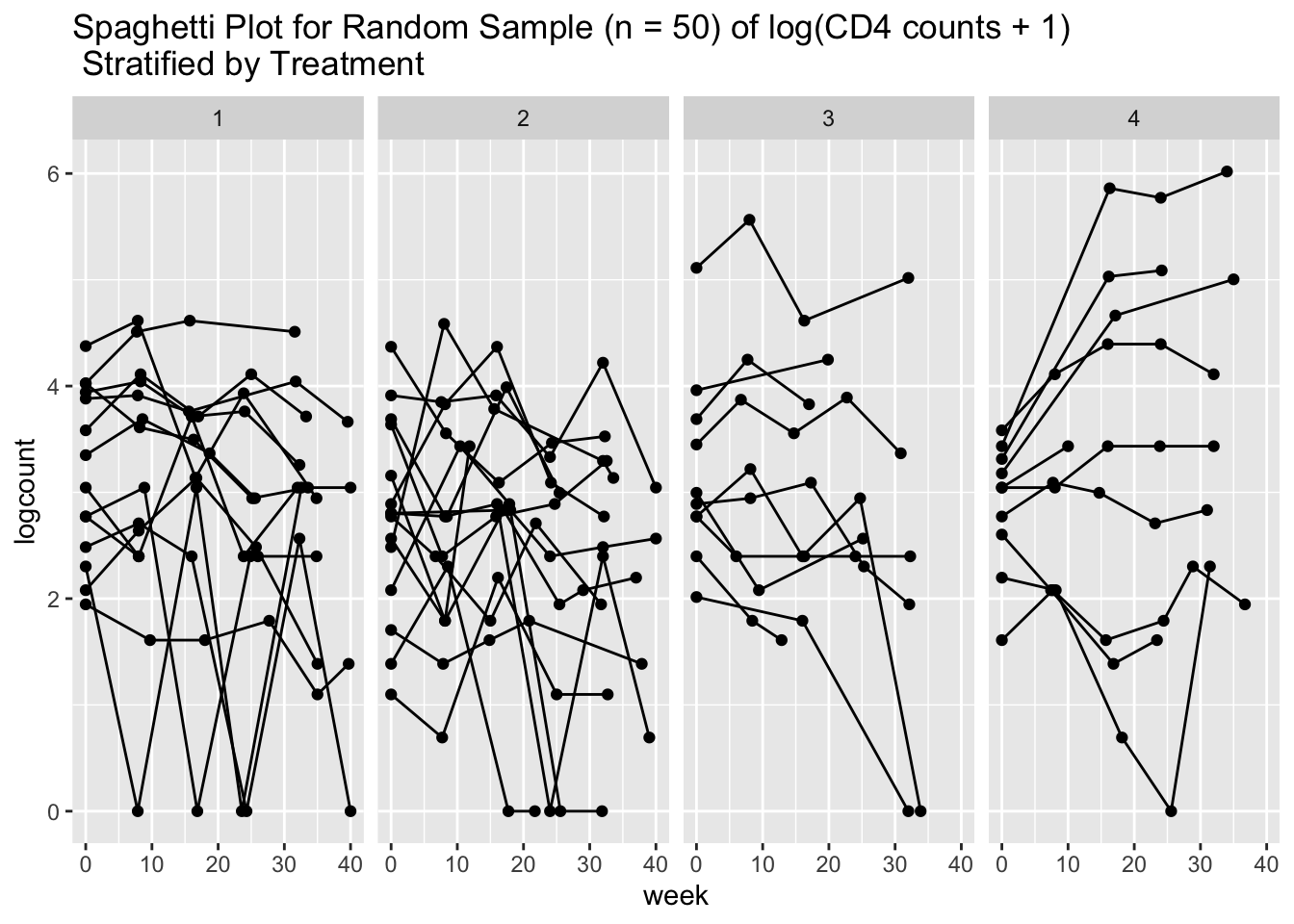

Figure 5.25: Spaghetti plot showing trajectories of a random sample of 50 individuals, stratified by treatment group.

We see from this small sample that individual trajectory varies greatly both between and within groups. We see non-linear time effects, and also differing slopes and intercepts within each treatment groups. This means we should consider random slope and intercept models that includes higher-orders of time and interactions that include the treatment group variable. We note that we must consider time as a continuous covariate in this setting because of the irregularity in the observation times.

When modelling the treatment, we will use treatment 4 as a reference as it’s the only triple therapy treatment. To do so, we start with a main-effects random slope and intercept model of the form \[ \mu_{ij} = \beta_0 + \beta_1\text{Trt1}_{ij} + \beta_2\text{Trt2}_{ij} + \beta_3\text{Trt3}_{ij} + \beta_4t_{ij} + b_{0,i} + b_{1,i}t_{ij} \] where \(\text{Trt1}_{ij} = 1\) if subject \(i\) is assigned to treatment 1 and = 0 otherwise, \(\text{Trt2}_{ij} = 1\) if subject \(i\) is assigned to treatment 2 and = 0 otherwise, \(\text{Trt3}_{ij} = 1\) if subject \(i\) is assigned to treatment 3 and = 0 otherwise, \(t_{ij}\) is the time of observation \(j\) for individual \(i\) (in weeks since baseline), and \(b_{0,i}\) and \(b_{1,i}\) are the random intercept and slope, respectively.

To begin, we assume an unstructured correlation structure for the random effects and independent structure for the within-subject correlation (default). We note that since we are interested in looking at the time trend specifically (fixed effect), we fit the model using the ML method. We fit this model with the following code:

# fit the random intercept and slope model
fitaids1 <- lme(
  fixed = logcount ~ T1 + T2 + T3 + week, # specify fixed effects
  random = ~ week | id, # random slope on time variable,
  # Intercept is included by default
  data = aidsdat,
  method = "ML"
) # default unstructured correlation for
# random effects and independence for within-subj correlation

We wish to compare this model with one that includes higher orders of time as well as interactions. We consider comparing the main-effects model against: \[ \begin{aligned} \mu_{ij} = \beta_0 &+ \beta_1\text{Trt1}_{ij} + \beta_2\text{Trt2}_{ij} + \beta_3\text{Trt3}_{ij} + \beta_4t_{ij} + \beta_5t_{ij}^2 + \\ &\beta_6\text{Trt1}_{ij}t_{ij} +\beta_7\text{Trt2}_{ij}t_{ij} + \beta_8\text{Trt4}_{ij}t_{ij} + \\ &\beta_9\text{Trt1}_{ij}t_{ij}^2 +\beta_{10}\text{Trt2}_{ij}t_{ij}^2 + \beta_{11}\text{Trt4}_{ij}t_{ij}^2 + \\ &b_{0,i} + b_{1,i}t_{ij} \end{aligned} \] In this model, we allow for a non-linear time trend that can vary between treatment groups. We leave the random effects as is, and will assess the structure of random effects after assessing the time trend. To fit this model in R, we first need to manually create the squared time variable and interactions. We note that again, we fit the model using the ML method.

#create squared time variable
aidsdat$weeksq <- (aidsdat$week)^2

#create all interactions
aidsdat$inter_T1week <- aidsdat$T1*aidsdat$week
aidsdat$inter_T2week <- aidsdat$T2*aidsdat$week
aidsdat$inter_T3week <- aidsdat$T3*aidsdat$week

aidsdat$inter_T1weeksq <- aidsdat$T1*aidsdat$weeksq
aidsdat$inter_T2weeksq <- aidsdat$T2*aidsdat$weeksq
aidsdat$inter_T3weeksq <- aidsdat$T3*aidsdat$weeksq

# fit the model
fitaids2 <- lme(
  fixed = logcount ~ T1 + T2 + T3 + week + weeksq +
    inter_T1week + inter_T2week + inter_T3week +
    inter_T1weeksq + inter_T2weeksq + inter_T3weeksq, # specify fixed effects
  random = ~ week | id, # random slope on time variable,
  # Intercept is included by default
  data = aidsdat,
  method = "ML"
) # default unstructured correlation for
# random effects and independence for within-subj correlation

The main effects model is nested in this model, and we have the same random effects present, so we can perform a LRT to see which model fits better. The null hypothesis is that the simpler model (fit1) fits as well as the fuller model (fit2). We do this in R by:

anova(fitaids1, fitaids2)

##          Model df      AIC      BIC    logLik   Test  L.Ratio p-value
## fitaids1     1  9 12110.30 12169.02 -6046.151                        
## fitaids2     2 16 11985.39 12089.78 -5976.694 1 vs 2 138.9134  <.0001

Our \(p\)-value is small, indicating that we reject the null hypothesis and conclude that the simpler model is not adequate.

We continue the model building process from this model.

Step 4: Consider Appropriate Random Effects Structure

Now that our time trend has been assessed, we focus on choosing the random effects. Our model is currently fit with an random intercept and random slope on our linear time effect. We can consider including other random covariates in our model at this stage.

First, as we included higher-order time terms, we can assess whether or not we should have a random effect on our weeksq variable. We fit a model including weeksq in the random = component of our model, and compare it to our original model using a modified LRT. We note that we cannot use the given \(p\)-value when comparing models with different random effects. As inference is on the random effects, we must re-fit the models using the REML estimation method.

# re-fit the model with only one random slope using REML
fitaids2_REML <- lme(
  fixed = logcount ~ T1 + T2 + T3 + week + weeksq +
    inter_T1week + inter_T2week + inter_T3week +
    inter_T1weeksq + inter_T2weeksq + inter_T3weeksq, # specify fixed effects
  random = ~ week | id, # random slope on time variable,
  # Intercept is included by default
  data = aidsdat,
  method = "REML"
) # default unstructured correlation for
# random effects and independence for within-subj correlation



# fit the new model with random slope on time and time^2
fitaids3_REML <- lme(
  fixed = logcount ~ T1 + T2 + T3 + week + weeksq +
    inter_T1week + inter_T2week + inter_T3week +
    inter_T1weeksq + inter_T2weeksq + inter_T3weeksq, # specify fixed effects
  random = ~ week + weeksq | id, # random slope on time and time^2 variable,
  # Intercept is included by default
  data = aidsdat,
  method = "REML"
) # default unstructured correlation for
# random effects and independence for within-subj correlation


# perform the modified LRT
LRT_mix_aids <- anova(fitaids3_REML, fitaids2_REML) #perform test
teststat_mix_aids <- LRT_mix_aids$L.Ratio[2] #grab test statistics
pchibarsq(teststat_mix_aids, df = 1, mix = 0.5) #degree of freedom is 1

## [1] 1

The large \(p\)-value indicates that we do not have evidence to reject the null hypothesis that the simpler model with only one random effect is better. As such, we can continue our analysis with the simpler model with a random intercept and random slope only on the linear time term (fitaids2).

Step 5: Variable Selection

Under the model above, we consider other fixed-effect variables at our disposal. In our model, we can consider age and gender as other covariates. We refit the model with these fixed effects and look at the model summary. We fit this model using the ML method as we are interested in the fixed effects.

# fit the model
# re-fit the model with only one random slope using REML
fitaids4 <- lme(
  fixed = logcount ~ T1 + T2 + T3 + week + weeksq + age + gender +
    inter_T1week + inter_T2week + inter_T3week +
    inter_T1weeksq + inter_T2weeksq + inter_T3weeksq, # specify fixed effects
  random = ~ week | id, # random slope on time variable,
  # Intercept is included by default
  data = aidsdat,
  method = "ML"
) # default unstructured correlation for
# random effects and independence for within-subj correlation

summary(fitaids4)

## Linear mixed-effects model fit by maximum likelihood
##   Data: aidsdat 
##        AIC      BIC    logLik
##   11976.97 12094.41 -5970.483
## 
## Random effects:
##  Formula: ~week | id
##  Structure: General positive-definite, Log-Cholesky parametrization
##             StdDev     Corr  
## (Intercept) 0.80125818 (Intr)
## week        0.01616871 0.18  
## Residual    0.57290009       
## 
## Fixed effects:  logcount ~ T1 + T2 + T3 + week + weeksq + age + gender + inter_T1week +      inter_T2week + inter_T3week + inter_T1weeksq + inter_T2weeksq +      inter_T3weeksq 
##                     Value  Std.Error   DF   t-value p-value
## (Intercept)     2.5496261 0.13909953 3719 18.329510  0.0000
## T1              0.0932740 0.07589996 1303  1.228907  0.2193
## T2              0.0849522 0.07581109 1303  1.120578  0.2627
## T3              0.0525470 0.07556476 1303  0.695391  0.4869
## week            0.0331363 0.00445349 3719  7.440537  0.0000
## weeksq         -0.0010068 0.00012212 3719 -8.243865  0.0000
## age             0.0106712 0.00307945 1303  3.465283  0.0005
## genderM        -0.0796127 0.07705184 1303 -1.033235  0.3017
## inter_T1week   -0.0461711 0.00641107 3719 -7.201772  0.0000
## inter_T2week   -0.0390965 0.00635733 3719 -6.149837  0.0000
## inter_T3week   -0.0260990 0.00636904 3719 -4.097786  0.0000
## inter_T1weeksq  0.0008925 0.00017706 3719  5.040844  0.0000
## inter_T2weeksq  0.0007545 0.00017415 3719  4.332539  0.0000
## inter_T3weeksq  0.0004848 0.00017621 3719  2.751460  0.0060
##  Correlation: 
##                (Intr) T1     T2     T3     week   weeksq age    gendrM
## T1             -0.264                                                 
## T2             -0.276  0.495                                          
## T3             -0.288  0.496  0.497                                   
## week           -0.129  0.240  0.240  0.241                            
## weeksq          0.107 -0.198 -0.198 -0.199 -0.925                     
## age            -0.788  0.003  0.005  0.017 -0.001  0.001              
## genderM        -0.397 -0.017  0.004  0.007 -0.002  0.002 -0.105       
## inter_T1week    0.087 -0.342 -0.167 -0.167 -0.695  0.643  0.004  0.001
## inter_T2week    0.090 -0.168 -0.339 -0.169 -0.701  0.648  0.003  0.000
## inter_T3week    0.094 -0.168 -0.168 -0.341 -0.699  0.647  0.001 -0.007
## inter_T1weeksq -0.072  0.282  0.137  0.137  0.638 -0.690 -0.002 -0.001
## inter_T2weeksq -0.075  0.139  0.280  0.140  0.649 -0.701 -0.002  0.001
## inter_T3weeksq -0.077  0.137  0.138  0.281  0.641 -0.693 -0.001  0.006
##                inter_T1wk inter_T2wk inter_T3wk intr_T1wks intr_T2wks
## T1                                                                   
## T2                                                                   
## T3                                                                   
## week                                                                 
## weeksq                                                               
## age                                                                  
## genderM                                                              
## inter_T1week                                                         
## inter_T2week    0.487                                                
## inter_T3week    0.486      0.490                                     
## inter_T1weeksq -0.925     -0.447     -0.446                          
## inter_T2weeksq -0.451     -0.924     -0.454      0.484               
## inter_T3weeksq -0.445     -0.449     -0.925      0.478      0.486    
## 
## Standardized Within-Group Residuals:
##         Min          Q1         Med          Q3         Max 
## -4.32307934 -0.43840832  0.03613471  0.48612402  3.58800387 
## 
## Number of Observations: 5036
## Number of Groups: 1309

We notice that the categorical gender variable has a large \(p\)-value, indicating it is not important to the model. We also notice that the stand-alone variables for treatments 1 to 3 are insignificant individually. We can test if these variables (which allow the log CD4 count to vary at baseline by treatment) are necessary.

We first re-fit the model without the gender variable:

# fit the model
fitaids5 <- lme(
  fixed = logcount ~ T1 + T2 + T3 + week + weeksq + age +
    inter_T1week + inter_T2week + inter_T3week +
    inter_T1weeksq + inter_T2weeksq + inter_T3weeksq, # specify fixed effects
  random = ~ week | id, # random slope on time variable,
  # Intercept is included by default
  data = aidsdat,
  method = "ML"
) # default unstructured correlation for
# random effects and independence for within-subj correlation

summary(fitaids5)

## Linear mixed-effects model fit by maximum likelihood
##   Data: aidsdat 
##        AIC      BIC    logLik
##   11976.03 12086.95 -5971.017
## 
## Random effects:
##  Formula: ~week | id
##  Structure: General positive-definite, Log-Cholesky parametrization
##             StdDev     Corr  
## (Intercept) 0.80139901 (Intr)
## week        0.01617039 0.183 
## Residual    0.57288806       
## 
## Fixed effects:  logcount ~ T1 + T2 + T3 + week + weeksq + age + inter_T1week +      inter_T2week + inter_T3week + inter_T1weeksq + inter_T2weeksq +      inter_T3weeksq 
##                     Value  Std.Error   DF   t-value p-value
## (Intercept)     2.4927063 0.12771463 3719 19.517782  0.0000
## T1              0.0919180 0.07588943 1304  1.211210  0.2260
## T2              0.0852870 0.07581145 1304  1.124988  0.2608
## T3              0.0530581 0.07556417 1304  0.702159  0.4827
## week            0.0331239 0.00445302 3719  7.438537  0.0000
## weeksq         -0.0010066 0.00012211 3719 -8.243094  0.0000
## age             0.0103336 0.00306341 1304  3.373251  0.0008
## inter_T1week   -0.0461640 0.00641042 3719 -7.201401  0.0000
## inter_T2week   -0.0390977 0.00635671 3719 -6.150622  0.0000
## inter_T3week   -0.0261423 0.00636826 3719 -4.105094  0.0000
## inter_T1weeksq  0.0008924 0.00017704 3719  5.040482  0.0000
## inter_T2weeksq  0.0007547 0.00017413 3719  4.333950  0.0000
## inter_T3weeksq  0.0004858 0.00017618 3719  2.757298  0.0059
##  Correlation: 
##                (Intr) T1     T2     T3     week   weeksq age    inter_T1wk
## T1             -0.295                                                     
## T2             -0.299  0.495                                              
## T3             -0.311  0.496  0.497                                       
## week           -0.141  0.240  0.240  0.241                                
## weeksq          0.117 -0.198 -0.198 -0.199 -0.925                         
## age            -0.909  0.002  0.005  0.017 -0.001  0.001                  
## inter_T1week    0.095 -0.342 -0.167 -0.167 -0.695  0.643  0.004           
## inter_T2week    0.097 -0.168 -0.339 -0.169 -0.701  0.648  0.002  0.487    
## inter_T3week    0.100 -0.168 -0.168 -0.340 -0.699  0.647  0.000  0.486    
## inter_T1weeksq -0.079  0.282  0.137  0.137  0.638 -0.690 -0.002 -0.925    
## inter_T2weeksq -0.081  0.139  0.280  0.140  0.649 -0.701 -0.002 -0.451    
## inter_T3weeksq -0.081  0.137  0.138  0.281  0.641 -0.693 -0.001 -0.445    
##                inter_T2wk inter_T3wk intr_T1wks intr_T2wks
## T1                                                        
## T2                                                        
## T3                                                        
## week                                                      
## weeksq                                                    
## age                                                       
## inter_T1week                                              
## inter_T2week                                              
## inter_T3week    0.490                                     
## inter_T1weeksq -0.447     -0.446                          
## inter_T2weeksq -0.924     -0.454      0.484               
## inter_T3weeksq -0.449     -0.925      0.478      0.486    
## 
## Standardized Within-Group Residuals:
##         Min          Q1         Med          Q3         Max 
## -4.32689940 -0.43909720  0.03549493  0.48585347  3.58573422 
## 
## Number of Observations: 5036
## Number of Groups: 1309

This model can be written as \[ \begin{aligned} \mu_{ij} = \beta_0 &+ \beta_1\text{Trt1}_{ij} + \beta_2\text{Trt2}_{ij} + \beta_3\text{Trt3}_{ij} + \beta_4t_{ij} + \beta_5t_{ij}^2 + \beta_6\text{age}_{ij} \\ &\beta_7\text{Trt1}_{ij}t_{ij} +\beta_8\text{Trt2}_{ij}t_{ij} + \beta_9\text{Trt4}_{ij}t_{ij} + \\ &\beta_{10}\text{Trt1}_{ij}t_{ij}^2 +\beta_{11}\text{Trt2}_{ij}t_{ij}^2 + \beta_{12}\text{Trt4}_{ij}t_{ij}^2 + \\ &b_{0,i} + b_{1,i}t_{ij} \end{aligned} \]

To test if the individual, stand-alone treatment variables are necessary in the model, we can test \(H_0: \beta_1 = \beta_2 = \beta_3 = 0\) vs \(H_A:\) at least one of these coefficients is non-zero. We can use the waldTestFunction presented in 5.4.8 to perform this test. We first create a matrix \(\bm{C}\) that will indicate the hypothesis test of interest. In our case, we want one column for each coefficient (including \(\beta_0\)) and one row for each coefficient in our hypothesis test. \[ \bm{C} = \begin{bmatrix} 0 & 1 & 0 & 0 & 0 & 0 & 0 & 0 & 0 & 0 & 0 & 0 & 0\\ 0 & 0 & 1 & 0 & 0 & 0 & 0 & 0 & 0 & 0 & 0 & 0 & 0\\ 0 & 0 & 0 & 1 & 0 & 0 & 0 & 0 & 0 & 0 & 0 & 0 & 0\\ \end{bmatrix}, \] In R, we create this matrix and perform the hypothesis test by:

C <- rbind(c(0,1,0,0,0,0,0,0,0,0,0,0,0),
           c(0,0,1,0,0,0,0,0,0,0,0,0,0),
           c(0,0,0,1,0,0,0,0,0,0,0,0,0))

waldTestFunction(C, fitaids5)

## 
##  Wald test chi-squared statistic is 1.846 with 3 df, p-value = 0.605 .

We fail to reject the null hypothesis and conclude that we do not need those terms in the model. As such, we can refit the model without those terms:

# fit the model
fitaids6 <- lme(
  fixed = logcount ~ week + weeksq + age +
    inter_T1week + inter_T2week + inter_T3week +
    inter_T1weeksq + inter_T2weeksq + inter_T3weeksq, # specify fixed effects
  random = ~ week | id, # random slope on time variable,
  # Intercept is included by default
  data = aidsdat,
  method = "ML"
) # default unstructured correlation for
# random effects and independence for within-subj correlation


summary(fitaids6)

## Linear mixed-effects model fit by maximum likelihood
##   Data: aidsdat 
##        AIC      BIC   logLik
##   11971.88 12063.22 -5971.94
## 
## Random effects:
##  Formula: ~week | id
##  Structure: General positive-definite, Log-Cholesky parametrization
##             StdDev    Corr  
## (Intercept) 0.8021100 (Intr)
## week        0.0161687 0.182 
## Residual    0.5729115       
## 
## Fixed effects:  logcount ~ week + weeksq + age + inter_T1week + inter_T2week +      inter_T3week + inter_T1weeksq + inter_T2weeksq + inter_T3weeksq 
##                     Value  Std.Error   DF   t-value p-value
## (Intercept)     2.5503002 0.11867209 3719 21.490312  0.0000
## week            0.0314956 0.00425444 3719  7.402995  0.0000
## weeksq         -0.0009696 0.00011840 3719 -8.189111  0.0000
## age             0.0103243 0.00306385 1307  3.369712  0.0008
## inter_T1week   -0.0435212 0.00602318 3719 -7.225622  0.0000
## inter_T2week   -0.0366747 0.00597912 3719 -6.133800  0.0000
## inter_T3week   -0.0246364 0.00598716 3719 -4.114881  0.0000
## inter_T1weeksq  0.0008323 0.00016983 3719  4.900474  0.0000
## inter_T2weeksq  0.0006998 0.00016712 3719  4.187267  0.0000
## inter_T3weeksq  0.0004517 0.00016907 3719  2.671707  0.0076
##  Correlation: 
##                (Intr) week   weeksq age    inter_T1wk inter_T2wk inter_T3wk
## week           -0.036                                                      
## weeksq          0.030 -0.921                                               
## age            -0.974 -0.004  0.003                                        
## inter_T1week   -0.005 -0.683  0.631  0.005                                 
## inter_T2week   -0.004 -0.689  0.636  0.004  0.486                          
## inter_T3week   -0.006 -0.687  0.635  0.006  0.486      0.489               
## inter_T1weeksq  0.004  0.623 -0.682 -0.003 -0.919     -0.444     -0.443    
## inter_T2weeksq  0.003  0.634 -0.693 -0.003 -0.448     -0.918     -0.450    
## inter_T3weeksq  0.006  0.626 -0.685 -0.006 -0.442     -0.446     -0.919    
##                intr_T1wks intr_T2wks
## week                                
## weeksq                              
## age                                 
## inter_T1week                        
## inter_T2week                        
## inter_T3week                        
## inter_T1weeksq                      
## inter_T2weeksq  0.483               
## inter_T3weeksq  0.478      0.486    
## 
## Standardized Within-Group Residuals:
##         Min          Q1         Med          Q3         Max 
## -4.32687871 -0.43823484  0.03516623  0.48710763  3.58566830 
## 
## Number of Observations: 5036
## Number of Groups: 1309

We can additionally make sure that the higher-order interaction terms are needed in the model:

# fit the model
fitaids7 <- lme(
  fixed = logcount ~ week + weeksq + age +
    inter_T1week + inter_T2week + inter_T3week , # specify fixed effects
  random = ~ week | id, # random slope on time variable,
  # Intercept is included by default
  data = aidsdat,
  method = "ML"
) # default unstructured correlation for
# random effects and independence for within-subj correlation


anova(fitaids6, fitaids7)

##          Model df      AIC      BIC    logLik   Test  L.Ratio p-value
## fitaids6     1 14 11971.88 12063.22 -5971.940                        
## fitaids7     2 11 11994.26 12066.03 -5986.132 1 vs 2 28.38466  <.0001

We reject the null hypothesis that the simpler model is adequate, and as such conclude that the model including the higher-order interaction terms is more appropriate.

We can also check to see if we should include higher-order terms of our age variable, or interactions between it and the treatment to see if there was a additional change in protein content of the milk produced by age within in each group. We first check if we should include age^2 in our model:

#create squared age variable
aidsdat$agesq <- (aidsdat$age)^2


fitaids8 <- lme(
  fixed = logcount ~ week + weeksq + age + agesq +
    inter_T1week + inter_T2week + inter_T3week +
    inter_T1weeksq + inter_T2weeksq + inter_T3weeksq, # specify fixed effects
  random = ~ week | id, # random slope on time variable,
  # Intercept is included by default
  data = aidsdat,
  method = "ML"
) # default unstructured correlation for
# random effects and independence for within-subj correlation

#compare to model 6 that does not include agesq variable
anova(fitaids6, fitaids8)

##          Model df      AIC      BIC    logLik   Test  L.Ratio p-value
## fitaids6     1 14 11971.88 12063.22 -5971.940                        
## fitaids8     2 15 11973.70 12071.56 -5971.849 1 vs 2 0.180606  0.6709

We fail to reject the null hypothesis that the simpler model (model 6, without the squared age term) fits as well as the model that includes the squared term. As such, we conclude that that term is not needed and continue model building from model 6.

Next, we check if we should have interactions between age and treatment. We first create the interaction term and see if they should be included in the model:

#create the interactions between age and treatment
aidsdat$inter_T1age <- aidsdat$age*aidsdat$T1
aidsdat$inter_T2age <- aidsdat$age*aidsdat$T2
aidsdat$inter_T3age <- aidsdat$age*aidsdat$T3


fitaids9 <- lme(
  fixed = logcount ~ week + weeksq + age + agesq +
    inter_T1week + inter_T2week + inter_T3week +
    inter_T1weeksq + inter_T2weeksq + inter_T3weeksq +
    inter_T1age + inter_T2age + inter_T3age, # specify fixed effects
  random = ~ week | id, # random slope on time variable,
  # Intercept is included by default
  data = aidsdat,
  method = "ML"
) # default unstructured correlation for
# random effects and independence for within-subj correlation

#compare to model 6 that does not include agesq variable
anova(fitaids6, fitaids9)

##          Model df      AIC      BIC    logLik   Test  L.Ratio p-value
## fitaids6     1 14 11971.88 12063.22 -5971.940                        
## fitaids9     2 18 11977.42 12094.86 -5970.712 1 vs 2 2.454881  0.6527

We again fail to reject the null hypothesis that the simpler model fits as well as the more complex model. As such, we should continue analysis with fitaids6 that includes the higher-order interaction terms between time (week) and treatment group, and a linear term for age.

Step 6: Model Diagnostics

As a final step, we assess the fit of this model. If the fit appears to be inadequate, we can iterate through the above procedure again. Detailed information on model diagnostics can be found in Section 5.4.6.

To assess if there is serial correlation among the random error term in our model, we can plot a variogram. We prefer to use a variogram instead of an ACF plot because we have irregularly spaced observations in our data set. To plot the variogram, we perform the following in R:

plot(Variogram(fitaids6, form = ~ week | id, collapse = "none",
     restype = "pearson", smooth = TRUE), xlab = "weeks", main = "Variogram Plot")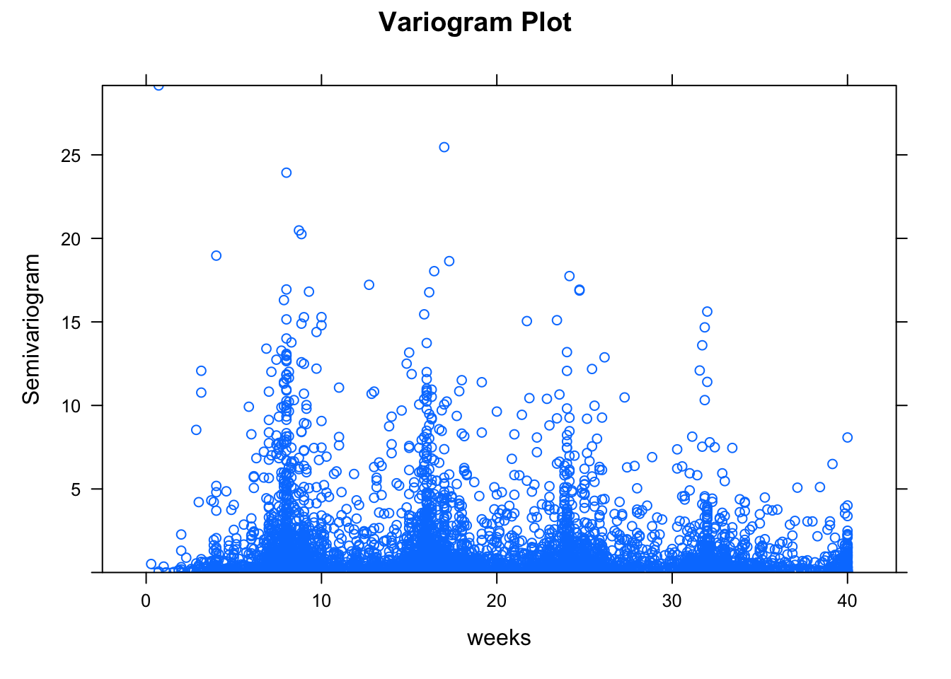

Figure 5.26: Variogram plot used to assess serial correlation in the fitted model: Model 6.

We look to see if there are any patterns or trends in the trend line, estimated by LOESS. It is difficult to see in this plot due to the number of observations, but the overall trend line is relatively flat and does not appear to increase or decrease over time. Most observations are low on the graph, indicating low degrees of serial correlation. As such, serial correlation is not an issue in this model.

Next, we check the common variances assumption by looking at a plot of the residuals. We do this in R by:

plot(residuals(fitaids6, type = "normalized"),  main = "Plot of Residuals for Model 6")

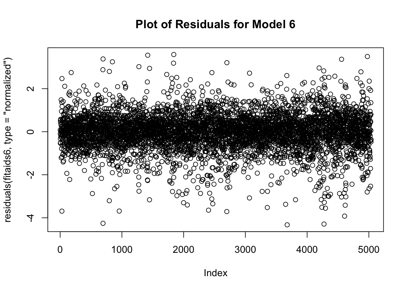
Figure 5.27: Residual plot for assessing the common variance assumption: Model 6

Most values here are within 2 standard deviations, and do not show any systematic patterns or clustering. This assumption appears to be satisfied.

Next, we check the normality of the errors through a Q-Q plot:

qqnorm(fitaids6, abline = c(0,1),
       main = "Q-Q Plot of Residuals")

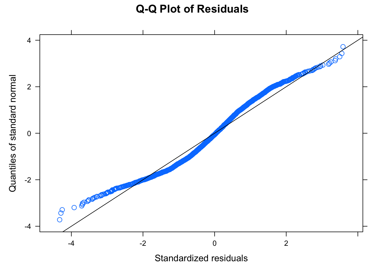
Figure 5.28: Plot for assessing normality of errors: Model 6

Here the Q-Q plot does not appear to be perfectly linear, however the majority of points are very close to the quantiles of the standard normal distribution. We conclude that the normality assumption here is satisfied.

Next, we look at the normality of the random intercept and slope:

qqnorm(fitaids6, ~ranef(.), 
       main = "Q-Q plot of Predicted Random Intercepts")

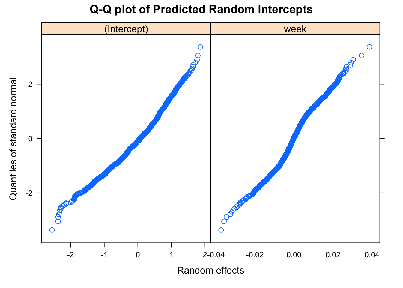
Figure 5.29: Plot for assessing normality of random slop andintercept.

Both plots appear to be relatively straight with no strange patterns or clustering, which indicates we have satisfied the normality assumption of the random effects.

Next, we assess linearity, which we can do my looking at the observed versus fitted values over the entire study population:

plot(fitaids6, logcount ~ fitted(.), abline = c(0,1),
     main = "Observed vs. Fitted Values")

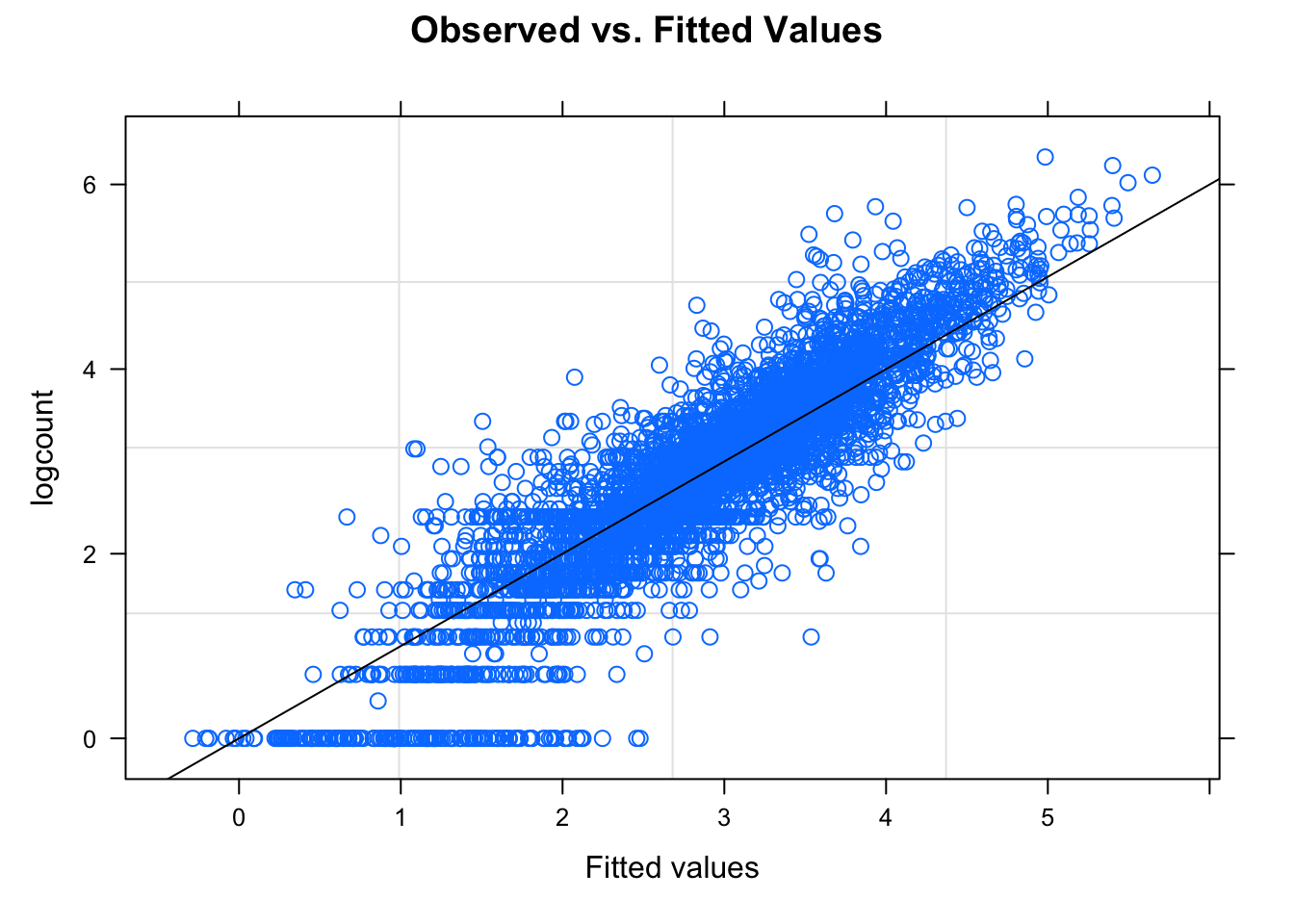
Figure 5.30: Plot for assessing linearity in the population.

Most observations appear to be linear. The banding in the bottom left corner is likely caused by the sample of individuals with log(1 + CD4 counts) = 0. We can also look at stratifying by treatment group:

plot(fitaids6, logcount ~ fitted(.)|treatment, abline = c(0,1),
     main = "Observed vs. Fitted Values")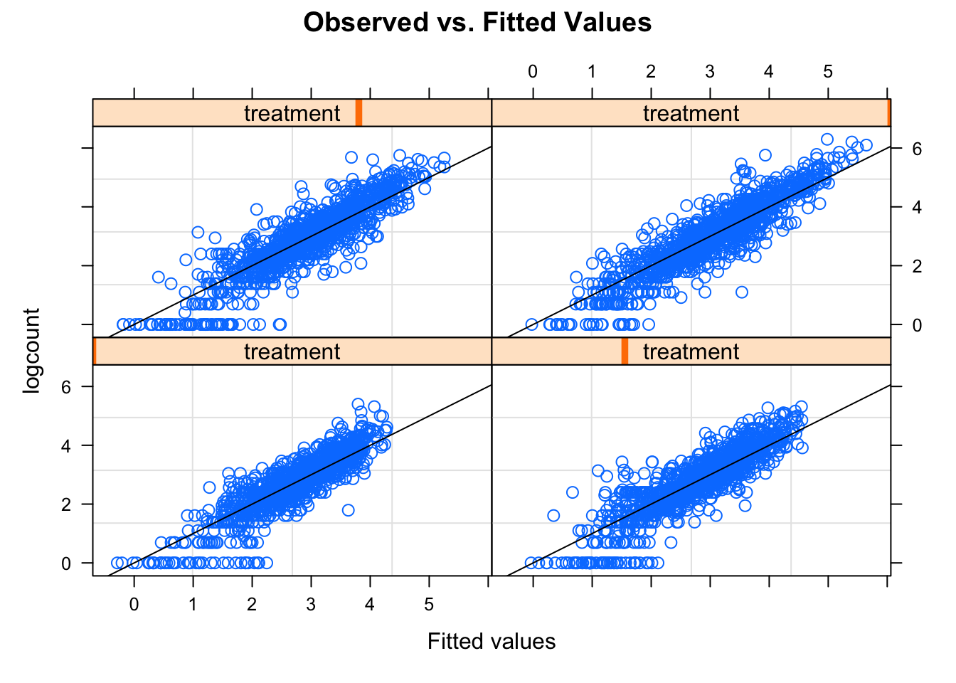

Figure 5.31: Plot for assessing linearity in each treatment.

Again, most observations appear to be linear. There are too many subjects to look at it on an individual level for the entire population.

Answering the Research Questions

Now that the assumptions have been satisfied, we can look at answering the research questions of interest. Let’s look at the model summary again:

summary(fitaids6)

## Linear mixed-effects model fit by maximum likelihood
##   Data: aidsdat 
##        AIC      BIC   logLik
##   11971.88 12063.22 -5971.94
## 
## Random effects:
##  Formula: ~week | id
##  Structure: General positive-definite, Log-Cholesky parametrization
##             StdDev    Corr  
## (Intercept) 0.8021100 (Intr)
## week        0.0161687 0.182 
## Residual    0.5729115       
## 
## Fixed effects:  logcount ~ week + weeksq + age + inter_T1week + inter_T2week +      inter_T3week + inter_T1weeksq + inter_T2weeksq + inter_T3weeksq 
##                     Value  Std.Error   DF   t-value p-value
## (Intercept)     2.5503002 0.11867209 3719 21.490312  0.0000
## week            0.0314956 0.00425444 3719  7.402995  0.0000
## weeksq         -0.0009696 0.00011840 3719 -8.189111  0.0000
## age             0.0103243 0.00306385 1307  3.369712  0.0008
## inter_T1week   -0.0435212 0.00602318 3719 -7.225622  0.0000
## inter_T2week   -0.0366747 0.00597912 3719 -6.133800  0.0000
## inter_T3week   -0.0246364 0.00598716 3719 -4.114881  0.0000
## inter_T1weeksq  0.0008323 0.00016983 3719  4.900474  0.0000
## inter_T2weeksq  0.0006998 0.00016712 3719  4.187267  0.0000
## inter_T3weeksq  0.0004517 0.00016907 3719  2.671707  0.0076
##  Correlation: 
##                (Intr) week   weeksq age    inter_T1wk inter_T2wk inter_T3wk
## week           -0.036                                                      
## weeksq          0.030 -0.921                                               
## age            -0.974 -0.004  0.003                                        
## inter_T1week   -0.005 -0.683  0.631  0.005                                 
## inter_T2week   -0.004 -0.689  0.636  0.004  0.486                          
## inter_T3week   -0.006 -0.687  0.635  0.006  0.486      0.489               
## inter_T1weeksq  0.004  0.623 -0.682 -0.003 -0.919     -0.444     -0.443    
## inter_T2weeksq  0.003  0.634 -0.693 -0.003 -0.448     -0.918     -0.450    
## inter_T3weeksq  0.006  0.626 -0.685 -0.006 -0.442     -0.446     -0.919    
##                intr_T1wks intr_T2wks
## week                                
## weeksq                              
## age                                 
## inter_T1week                        
## inter_T2week                        
## inter_T3week                        
## inter_T1weeksq                      
## inter_T2weeksq  0.483               
## inter_T3weeksq  0.478      0.486    
## 
## Standardized Within-Group Residuals:
##         Min          Q1         Med          Q3         Max 
## -4.32687871 -0.43823484  0.03516623  0.48710763  3.58566830 
## 
## Number of Observations: 5036
## Number of Groups: 1309

This model can be written as: \[ \begin{aligned} \mu_{ij} = \beta_0 &+ \beta_1t_{ij} + \beta_2t_{ij}^2 + \beta_3\text{age}_{ij} \\ &\beta_4\text{Trt1}_{ij}t_{ij} +\beta_5\text{Trt2}_{ij}t_{ij} + \beta_6\text{Trt4}_{ij}t_{ij} + \\ &\beta_{7}\text{Trt1}_{ij}t_{ij}^2 +\beta_{8}\text{Trt2}_{ij}t_{ij}^2 + \beta_{9}\text{Trt4}_{ij}t_{ij}^2 + \\ &b_{0,i} + b_{1,i}t_{ij} \end{aligned} \]

We are interested in seeing if the change in log-transformed CD4 counts (log(CD4 counts + 1)) from baseline varied between treatment groups, with increased interest in the effect of the dual vs triple combination treatments. Based on this model, we have statistically significant interaction terms that indicate that the time trend of log(1 + CD4 counts) varies by treatment group.

From the fitaids6 model, we conclude that the change in log(1 + CD4 counts) from baseline varies by treatment groups, with a non-linear trend, particularly for the triple therapy treatment (treatment 4). We also note that age is significantly associated with increased log(1 + CD4 counts), controlling for treatment allocation and the time effect.

We note that we are also interested in seeing if there is a difference between the dual and triple therapies. To investigate this hypothesis, we can create a new variable that represents the individual was assigned to treatment 4 (triple therapy) or not (dual).

# Create triple treatment indicator
aidsdat$triple <- ifelse(aidsdat$treatment == 4, 1, 0)

# Create interaction terms
aidsdat$inter_tripleweek <- aidsdat$triple*aidsdat$week
aidsdat$inter_tripleweeksq <- aidsdat$triple*aidsdat$weeksq


# fit the model
fitaids6_combtreatments <- lme(
  fixed = logcount ~ week + weeksq + age +
    inter_tripleweek + inter_tripleweeksq, # specify fixed effects
  random = ~ week | id, # random slope on time variable,
  # Intercept is included by default
  data = aidsdat,
  method = "ML"
) # default unstructured correlation for
# random effects and independence for within-subj correlation


summary(fitaids6_combtreatments)

## Linear mixed-effects model fit by maximum likelihood
##   Data: aidsdat 
##        AIC      BIC    logLik
##   11976.54 12041.79 -5978.271
## 
## Random effects:
##  Formula: ~week | id
##  Structure: General positive-definite, Log-Cholesky parametrization
##             StdDev     Corr  
## (Intercept) 0.80201054 (Intr)
## week        0.01627928 0.185 
## Residual    0.57344311       
## 
## Fixed effects:  logcount ~ week + weeksq + age + inter_tripleweek + inter_tripleweeksq 
##                         Value  Std.Error   DF   t-value p-value
## (Intercept)         2.5502189 0.11869448 3723 21.485572  0.0000
## week               -0.0033565 0.00259880 3723 -1.291575  0.1966
## weeksq             -0.0003105 0.00007228 3723 -4.295298  0.0000
## age                 0.0103217 0.00306450 1307  3.368134  0.0008
## inter_tripleweek    0.0348610 0.00486959 3723  7.158933  0.0000
## inter_tripleweeksq -0.0006594 0.00013657 3723 -4.828543  0.0000
##  Correlation: 
##                    (Intr) week   weeksq age    inter_trplwk
## week               -0.072                                  
## weeksq              0.059 -0.923                           
## age                -0.974  0.005 -0.004                    
## inter_tripleweek    0.007 -0.487  0.454 -0.006             
## inter_tripleweeksq -0.005  0.451 -0.498  0.005 -0.919      
## 
## Standardized Within-Group Residuals:
##         Min          Q1         Med          Q3         Max 
## -4.31270016 -0.44144321  0.03870598  0.48492477  3.58419390 
## 
## Number of Observations: 5036
## Number of Groups: 1309

Under this parameterization, we do see that the interaction terms are individually significant. This indicates that there is a difference in time trend by dual versus triple therapy, controlling for age. For example, we see that the effect of time on the triple action treatment on log(CD4 counts + 1) is greater by 0.035 units compared to dual action therapy, controlling for age. We also see that the squared time effect interaction is significant but the effect size is small (-0.001). We can interpret this that the effect of the squared time term on log(CD4 counts + 1) is smaller by 0.001 units for the triple action therapy compared to dual action therapy.

We can see if this model is more adequate, indicating that treatments 1, 2, and 3 have the same treatment effect over time.

anova(fitaids6, fitaids6_combtreatments)

##                         Model df      AIC      BIC    logLik   Test  L.Ratio
## fitaids6                    1 14 11971.88 12063.22 -5971.940                
## fitaids6_combtreatments     2 10 11976.54 12041.79 -5978.271 1 vs 2 12.66315
##                         p-value
## fitaids6                       
## fitaids6_combtreatments   0.013

We reject the null hypothesis that the model that combines treatments 1, 2 and 3 is adequate compared to the original model. This indicates that there exists at least one dual-treatment therapy that has a different time effect on the log(1 + CD4 counts). Looking at the LOESS curves from Figure 5.24, this is unsurprising as treatment 3 appears to have a different time trend than treatments 1 and 2, which are similar.

References

Diggle, Peter J., Patrick Heagerty, Kung-Yee Liang, and Scott L. Zeger. 2002. Analysis of Longitudinal Data. 2nd ed. Oxford, UK: Oxford University Press.

Fitzmaurice, Garrett M., Nan M. Laird, and James H. Ware. 2011. Applied Longitudinal Analysis. 2nd ed. Hoboken, NJ: Wiley.