Generalized Box-Cox transformation.

Generalized Box-Cox transformation.

powTrans(x, lambda = 0, alpha = 0, normalize = FALSE,
  jacobian = FALSE)

Arguments

x	Vector of quantiles at which to compute the transformation.
lambda	Exponent of the transformation. See Details.
alpha	Offset of the transformation. See Details.
normalize	Logical; if TRUE divides by the geometric mean. See Details.
jacobian	Logical; if TRUE calculates the Jacobian |dz / dx|, which converts transformed density values back to the original scale.

Value

The vector z of transformed values, and optionally the Jacobian of the inverse transformation. See Details.

Details

The Generalized Power or Box-Cox transformation is $$ z = \begin{array}{rl} ((x + \alpha)^\lambda - 1) / (\lambda C^{\lambda-1}) & \lambda \neq 0 \\ C \log(x + \alpha) & \lambda = 0, \end{array} $$

where \(C\) is the Geometric mean, i.e., C = exp(mean(log(x + alpha))). Note that C is only calculated if normalize = TRUE.

Examples

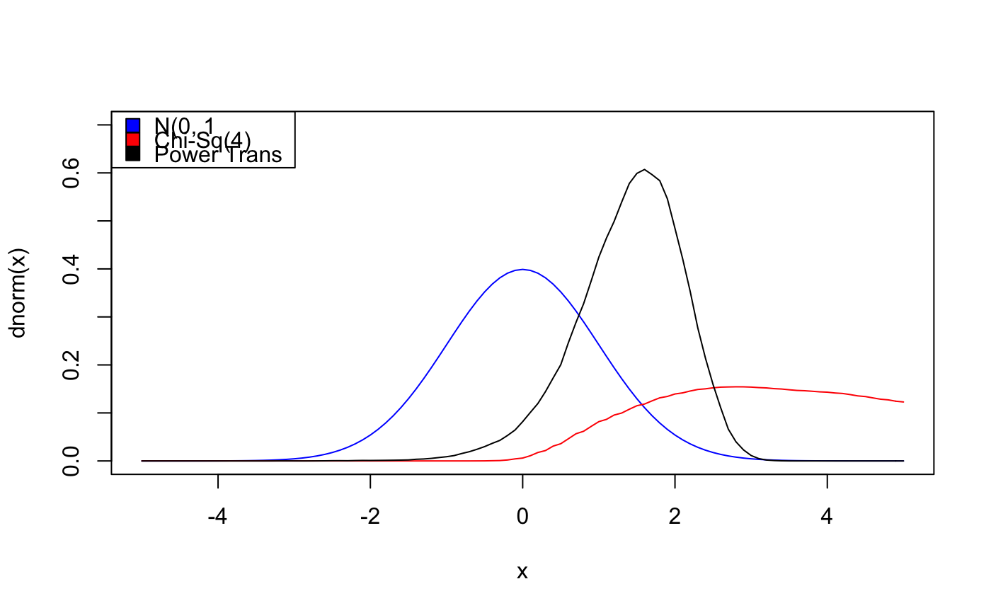
# generate data and plot
# apply power transform and superimpose on plot
# finally, superimpose N(0, 1) on plot
n <- 1e5
df <- 5
X <- rchisq(n, df = df)
xdens <- kernelXD(X)
xdens.trans <- kernelXD(powTrans(X))
# plots
curve(dnorm(x), col = "blue", xlim=c(-5, 5), ylim = c(0,0.7)) # true PDF
curve(dXD(x, xDens = xdens), add = TRUE, col = "red") # xDensity PDF
curve(dXD(x, xDens = xdens.trans), add = TRUE, col = "black") # xDensity PDF
legend("topleft", c("N(0, 1", "Chi-Sq(4)", "Power Trans"),
       pch = c(22,22,22,NA), pt.cex = 1.5,
       pt.bg = c("blue", "red", "black"))