Graphical and numerical checks for mode-finding routines.

Tools for checking that the output of an optimization algorithm is indeed at a local mode of the objective function. This is accomplished graphically by calculating all one-dimensional "projection plots" of the objective function, i.e., varying each input variable one at a time with all other elements of the potential solution being fixed. The numerical values in these plots can be readily extracted for the purpose of automated and systematic unit-testing of optimization routines.

See also

Useful links:

• https://github.com/mlysy/optimCheck

• Report bugs at https://github.com/mlysy/optimCheck/issues

Author

Maintainer: Martin Lysy mlysy@uwaterloo.ca

Examples

# example: logistic regression
ilogit <- binomial()$linkinv

# generate data
p <- sample(2:10,1) # number of parameters
n <- sample(1000:2000,1) # number of observations
X <- matrix(rnorm(n*p),n,p) # design matrix
beta0 <- rnorm(p, sd = .1) # true parameter values
y <- rbinom(n, size = 1, prob = ilogit(X %*% beta0)) # response

# fit logistic regression
bhat <- coef(glm(y ~ X - 1, family = binomial))

# check convergence

# likelihood function
loglik <- function(beta, y, X) {
  sum(dbinom(y, size = 1, prob = ilogit(X %*% beta), log = TRUE))
}

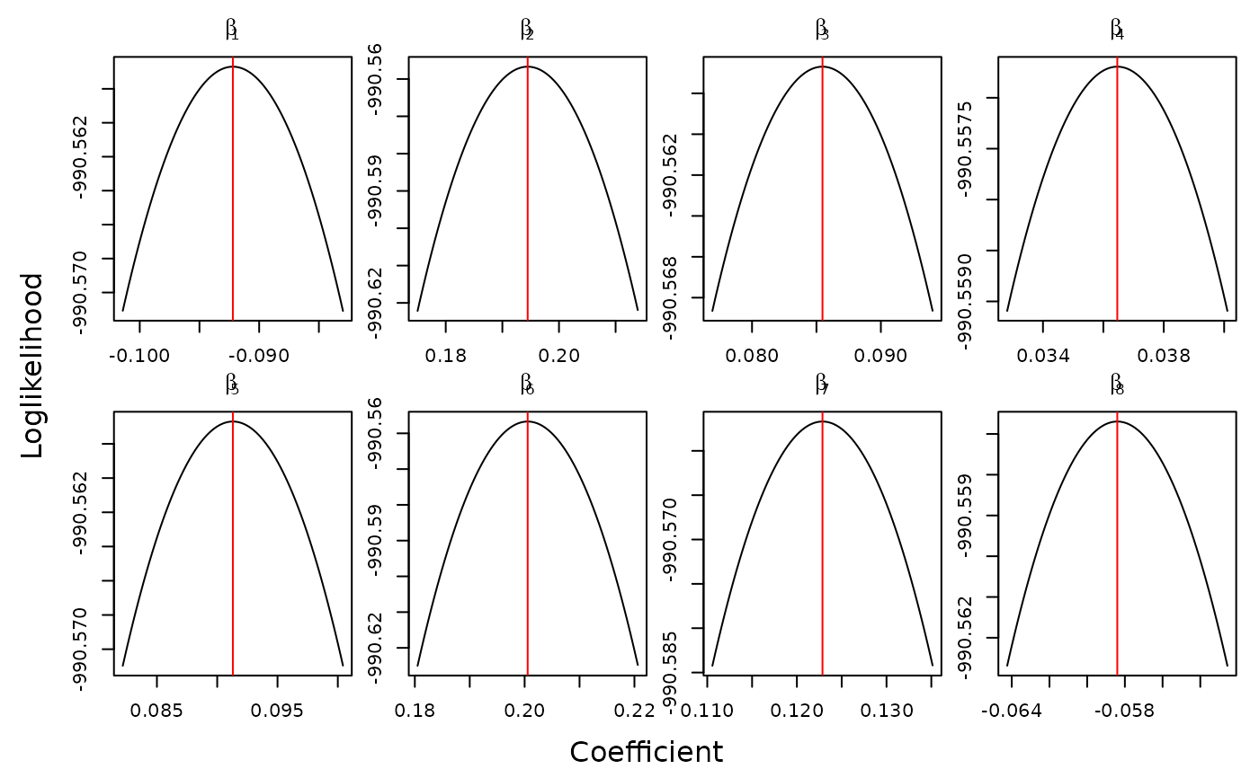
# projection plots
bnames <- parse(text = paste0("beta[", 1:p, "]"))
system.time({
  oproj <- optim_proj(xsol = bhat,
                      fun = function(beta) loglik(beta, y, X),
                      xnames = bnames,
                      xlab = "Coefficient", ylab = "Loglikelihood")
})

#>    user  system elapsed 
#>   0.207   0.417   0.163 

# numerical summary
oproj # see ?summary.optproj for more information
#> 
#> 'optim_proj' check on 8-variable maximization problem.
#> 
#> Top 5 relative errors in potential solution:
#> 
#>        xsol D=xopt-xsol R=D/|xsol|
#> X1 -0.09220  -9.313e-05   -0.00101
#> X2  0.19450   1.964e-04    0.00101
#> X3  0.08547   8.633e-05    0.00101
#> X4  0.03646   3.683e-05    0.00101
#> X5  0.09130   9.222e-05    0.00101
#> 

# elementwise differences between potential and optimal solution
diff(oproj) # same as summary(oproj)$xdiff
#>              abs          rel
#> X1 -9.313317e-05 -0.001010101
#> X2  1.964355e-04  0.001010101
#> X3  8.633245e-05  0.001010101
#> X4  3.682969e-05  0.001010101
#> X5  9.222004e-05  0.001010101
#> X6  2.025807e-04  0.001010101
#> X7  1.240967e-04  0.001010101
#> X8 -5.899198e-05 -0.001010101

# refit general purpose optimizer starting from bhat
# often faster than optim_proj, but less stable
system.time({
  orefit <- optim_refit(xsol = bhat,
                        fun = function(beta) loglik(beta, y, X))
})
#>    user  system elapsed 
#>   0.022   0.024   0.012 
orefit
#> 
#> 'optim_refit' check on 8-variable maximization problem.
#> 
#> Top 5 relative errors in potential solution:
#> 
#>        xsol D=xopt-xsol R=D/|xsol|
#> X1 -0.09220           0          0
#> X2  0.19450           0          0
#> X3  0.08547           0          0
#> X4  0.03646           0          0
#> X5  0.09130           0          0
#>