Quick Tour of Package **optimCheck** • optimCheck

Introduction

The optimCheck package provides a set of tools to check that output of an optimization algorithm is indeed at a local mode of the objective function. The tools include both visual and numerical checks, the latter serving to automate formalized unit tests with e.g., the R packages testthat or RUnit.

Example: Quadratic Objective Function

A brief overview of the package functionality is illustrated with the following example. Let $Q(\boldsymbol{x}) = \boldsymbol{x}'\boldsymbol{A}\boldsymbol{x}- 2 \boldsymbol{b}'\boldsymbol{x}$ denote a quadratic objective function in $\boldsymbol{x}\in \mathbb R^d$ . If $\boldsymbol{A}_{d \times d}$ is a positive-definite matrix, then the unique minimum of $Q(\boldsymbol{x})$ is $\hat{\boldsymbol{x}}= \boldsymbol{A}^{-1}\boldsymbol{b}$ . Let us now ignore this information and try to minimize $Q(\boldsymbol{x})$ using R’s simplest built-in mode-finding routine, provided by the R function stats::optim().

In its simplest configuration, stats::optim() requires only the objective function and a starting value $\boldsymbol{x}_0$ to initialize the mode-finding procedure. Let’s consider a difficult setting for stats::optim(), with a relatively large $d = 12$ and a starting value $\boldsymbol{x}_0$ which is far from the optimal value $\hat{\boldsymbol{x}}$ .

d <- 12 # dimension of optimization problem

# create the objective function: Q(x) = x'Ax - 2b'x
A <- crossprod(matrix(rnorm(d^2), d, d)) # positive definite matrix
b <- rnorm(d)
objfun <- function(x) crossprod(x, A %*% x)[1] - 2 * crossprod(b, x)[1]

xhat <- solve(A, b) # analytic solution

# numerical mode-finding using optim
xfit <- optim(fn = objfun,                    # objective function
              par = xhat * 5,                 # initial value is far from the solution
              control = list(maxit = 1e5))    # very large max. number of iterations

Visual Checks with `optim_proj()`

Like most solvers, stats::optim() utilizes various criteria to determine whether its algorithm has converged, which can be assess with the following command:

# any value other than 0 means optim failed to converge
xfit$convergence

## [1] 0

Here stats::optim() reports that its algorithm has converged. Now let’s check this visually with optimCheck using projection plots. That is, let $\tilde{\boldsymbol{x}}$ denote the potential optimum of $Q(\boldsymbol{x})$ . Then for each $i = 1,\ldots,d$ , we plot $Q_i(x_i) = Q(x_i, \tilde{\boldsymbol{x}}_{-i}), \qquad \tilde{\boldsymbol{x}}_{-i} = (\tilde x_1, \ldots, \tilde x_{i-1}, \tilde x_{i+1}, \ldots, \tilde x_d).$ In other words, projection plot $i$ varies only $x_i$ , while holding all other elements of $\boldsymbol{x}$ fixed at the value of the potential solution $\tilde{\boldsymbol{x}}$ . These plots are produced with the optimCheck function optim_proj():

require(optimCheck) # load package

## Loading required package: optimCheck

# projection plots
xnames <- parse(text = paste0("x[", 1:d, "]")) # variable names
oproj <- optim_proj(fun = objfun,              # objective function
                    xsol = xfit$par,           # potential solution
                    maximize = FALSE,          # indicates that a local minimum is sought
                    xrng = .5,                 # range of projection plot: x_i +/- .5*|x_i|
                    xnames = xnames)

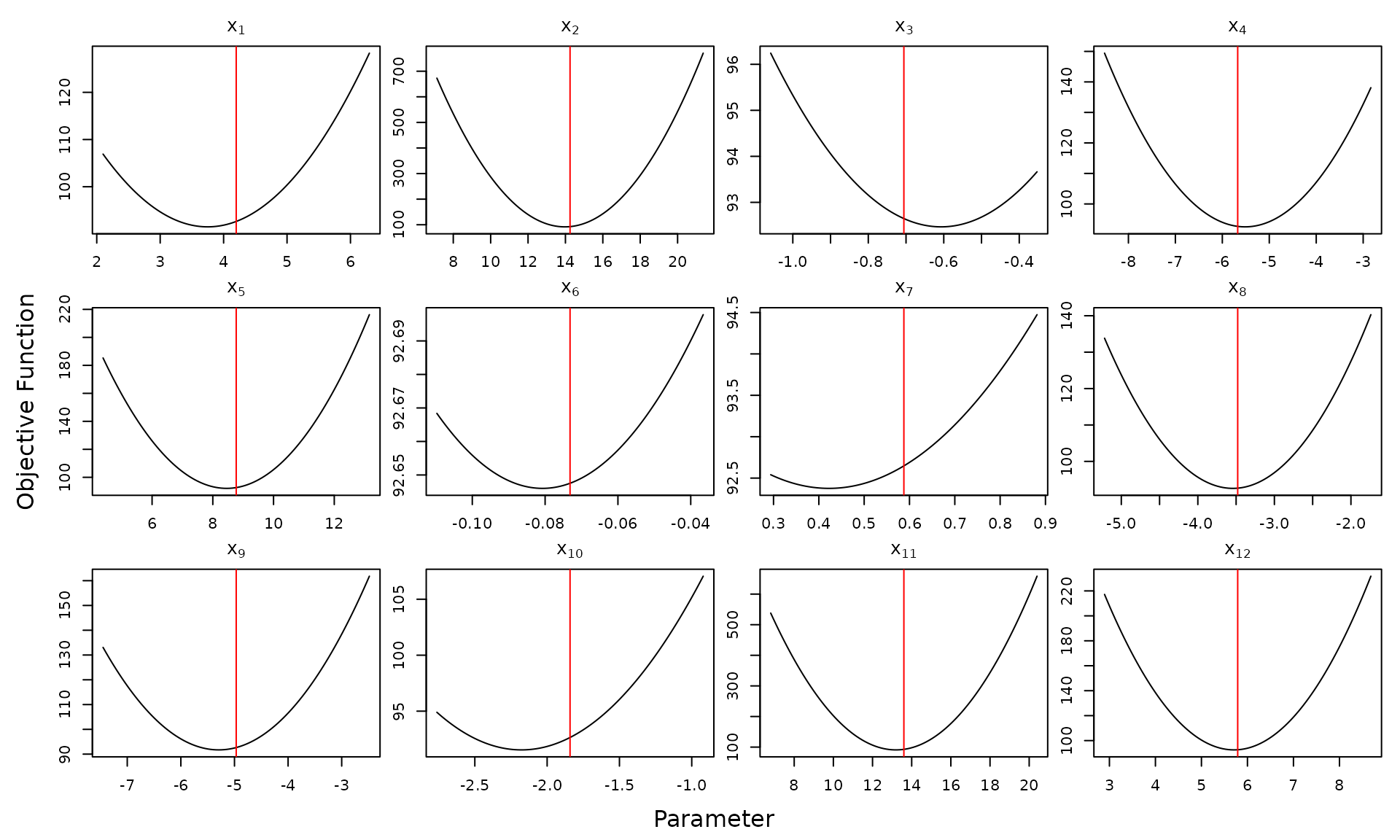
In each of the projection plots, the potential solution $\tilde x_i$ is plotted in red. The xrng argument to optim_proj() specifies the plotting range. Among various ways of doing this, perhaps the simplest is a single scalar value indicating that each plot should span $x_i \pm$ xrng $\cdot |x_i|$ . Thus we can see from these plots that stats::optim() was sometimes up to 10% away from the local mode of the projection plots.

Quantification of Projection Plots

Projection plots are a powerful method of assessing the convergence of mode-finding routines to a local mode. While great for interactive testing, plots are not well-suited to automated unit testing as part of an R package development process. To this end, optimCheck provides a means of quantifying the result of a call to optim_proj(). Indeed, a call to optim_proj() returns an object of class optproj with the following elements:

sapply(oproj, function(x) dim(as.matrix(x)))

##      xsol ysol maximize xproj yproj
## [1,]   12    1        1   100   100
## [2,]    1    1        1    12    12

As described in the function documentation, xproj and yproj are matrices of which each column contains the $x$ -axis and $y$ -axis coordinates of the points contained in each projection plot. The summary() method for optproj objects coverts these to absolute and relative errors in both the potential solution and the objective function. The print() method conveniently displays these results:

oproj # same print method as summary(oproj)

## 
## 'optim_proj' check on 12-variable minimization problem.
## 
## Top 5 relative errors in potential solution:
## 
##         xsol D=xopt-xsol R=D/|xsol|
## x7   0.58760   -0.163200    -0.2778
## x10 -1.84200   -0.344100    -0.1869
## x3  -0.70570    0.096230     0.1364
## x1   4.19900   -0.445300    -0.1061
## x6  -0.07315   -0.007758    -0.1061

The documentation for summary.optproj() describes the various calculations it provides. Perhaps the most useful of these are the elementwise absolute and relative differences between the potential solution $\tilde{\boldsymbol{x}}$ and $\hat{\boldsymbol{x}}_\mathrm{proj}$ , the vector of optimal 1D solutions in each projection plot. For convenience, these can be extracted with the diff() method:

diff(oproj) # equivalent to summary(oproj)$xdiff

##              abs         rel
## x1  -0.445321028 -0.10606061
## x2  -0.215858067 -0.01515152
## x3   0.096231561  0.13636364
## x4   0.143242614  0.02525253
## x5  -0.310081433 -0.03535354
## x6  -0.007758386 -0.10606061
## x7  -0.163226011 -0.27777778
## x8  -0.052715576 -0.01515152
## x9  -0.326153891 -0.06565657
## x10 -0.344134419 -0.18686869
## x11 -0.343453576 -0.02525253
## x12 -0.087700503 -0.01515152

# here's exactly what these are
xsol <- summary(oproj)$xsol # candidate solution
xopt <- summary(oproj)$xopt # optimal solution in each projection plot
xdiff <- cbind(abs = xopt-xsol, rel = (xopt-xsol)/abs(xsol))
range(xdiff - diff(oproj))

## [1] 0 0

Thus it is proposed that a combination of summary() and diff() methods for projection plots can be useful for constructing automated unit tests. In this case, plotting itself can be disabled by passing optim_proj() the argument plot = FALSE. See the optimCheck/tests folder for testthat examples featuring:

Logistic Regression (stats::glm() function).
Quantile Regression (quantreg::rq() function in quantreg)
Multivariate normal mixtures (mclust::emEEE() in mclust).

You can run these tests with the command

testthat::test_package("optimCheck", reporter = "progress")

`optim_refit()`: A Numerical Alternative to Projection Plots

There are some situations in which numerical quantification of projection plots leaves to be desired:

Generating all projection plots requires N = 2 * npts * length(xsol) evaluations of the objective function (where the default value is npts = 100), which can belabor the process of automated unit testing. A different test for mode-finding routines is to recalculate the optimal solution with an “very good” starting point: the current potential solution. This is the so-called “refine optizimation” – or refit – strategy.

The optim_refit() function refines the optimization with a call to R’s built-in general-purpose optimizer: the function stats::optim(). In particular, it selects the default Nelder-Mead simplex method with a simplified parameter interface. As seen in the unit tests above, the refit checks are 2-3 times faster than their projection plot counterparts. Consider now the example of refining the original stats::optim() solution to the quadratic objective function:

orefit <- optim_refit(fun = objfun,        # objective function
                      xsol = xfit$par,     # potential solution
                      maximize = FALSE)    # indicates that a local minimum is sought

## Warning in optim_refit(fun = objfun, xsol = xfit$par, maximize = FALSE):
## Iteration limit maxit has been reached.

summary(orefit) # same print method as orefit

## 
## 'optim_refit' check on 12-variable minimization problem.
## 
## Top 5 relative errors in potential solution:
## 
##          xsol D=xopt-xsol R=D/|xsol|
## [1,]  0.58760     -1.5230     -2.592
## [2,] -0.70570      1.5430      2.186
## [3,] -1.84200      3.0410      1.651
## [4,] -0.07315     -0.1021     -1.396
## [5,]  4.19900     -4.2820     -1.020

Thus we can see that the first and second run of stats::optim() are quite different.

Of course, this does not mean that the refit solution produced by stats::optim() is a local mode:

# projection plots with refined solution
optim_proj(xsol = orefit$xopt, fun = objfun,
           xrng = .5, maximize = FALSE)

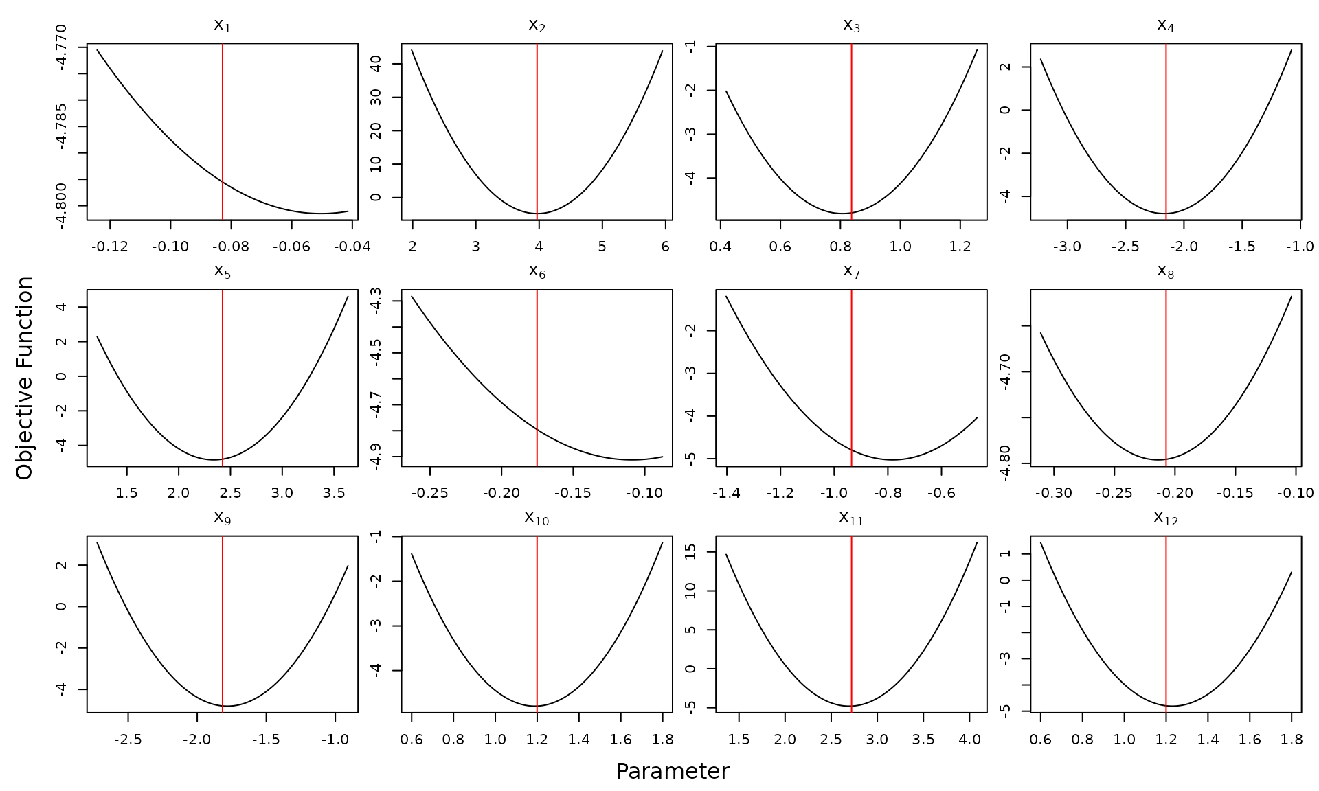
Indeed, the default stats::optim() method is only accurate when initialized close to the optimal solution. Therefore, one may wish to run the refit test with a different optimizer. This can be done externally to optim_refit, prior to passing the refit solution to the function via its argument xopt. This is illustrated below using stats::optim()’s gradient-based quasi-Newton method:

# gradient of the objective function
objgrad <- function(x) 2 * drop(A %*% x - b)

# mode-finding using quasi-Newton method
xfit2 <- optim(fn = objfun,                    # objective function
               gr = objgrad,                   # gradient
               par = xfit$par,                 # initial value (first optim fit)
               method = "BFGS")

# external refit test with optimizer of choice
orefit2 <- optim_refit(fun = objfun,
                       xsol = xfit$par,        # initial value (first optim fit)
                       xopt = xfit2$par,       # refit value (2nd fit with quasi-Newton method
                       maximize = FALSE)

# project plot test on refit solution
optim_proj(xsol = orefit2$xopt, fun = objfun,
           xrng = .5, maximize = FALSE, plot = FALSE)

## 
## 'optim_proj' check on 12-variable minimization problem.
## 
## Top 5 relative errors in potential solution:
## 
##       xsol D=xopt-xsol R=D/|xsol|
## x1  0.5008   -0.002530  -0.005051
## x2  3.0600   -0.015450  -0.005051
## x3 -0.3098    0.001564   0.005051
## x4 -1.4320    0.007233   0.005051
## x5  1.5770    0.007967   0.005051

Future Work: Constrained Optimization

Many constrained statistical optimization problems, seek a “sparse” solution, i.e., one for which some of the elements of the optimal solution are equal to zero. In such cases, the relative difference between potential and optimal solution is an unreliable metric. A working proposal is to flag these “true zeros” in optim_proj() and optim_refit(), so as to add a 1 to the relative difference denominators. Other suggestions on this and optimCheck in general are welcome.

Quick Tour of Package optimCheck

Martin Lysy

2024-09-05

Introduction

Example: Quadratic Objective Function

Visual Checks with `optim_proj()`

Quantification of Projection Plots

`optim_refit()`: A Numerical Alternative to Projection Plots

Future Work: Constrained Optimization

Quick Tour of Package optimCheck

Martin Lysy

2024-09-05

Introduction

Example: Quadratic Objective Function

Visual Checks with optim_proj()

Quantification of Projection Plots

optim_refit(): A Numerical Alternative to Projection Plots

Future Work: Constrained Optimization

Visual Checks with `optim_proj()`

`optim_refit()`: A Numerical Alternative to Projection Plots