Gibbs sampler for posterior distribution of parameters and hyperparameters of a multivariate normal random-effects linear regression model called RxNormLM (see Details).
RxNormLM(
  nsamples,
  Y,
  V,
  X,
  prior = NULL,
  init,
  burn,
  updateHyp = TRUE,
  storeHyp = TRUE,
  updateRX = TRUE,
  storeRX = FALSE
)
Arguments
- nsamples
number of posterior samples to draw.
- Y
N x qmatrix of responses.- V
Either a
q x qvariance matrix or anq x q x Narray of such matrices.- X
N x pmatrix of covariates.- prior
parameters of the prior MNIW distribution on the hyperparameters (see Details).
- init
(optional) list with elements
Beta,Sigma, andMuproviding the initial values for these. Default values areBeta = matrix(0, p, q),Sigma = diag(q), andMu = Y.- burn
integer number of burn-in samples, or fraction of
nsamplesto prepend as burn-in.- updateHyp, storeHyp
logical. Whether or not to update/store the hyperparameter draws.
- updateRX, storeRX
logical. Whether or not to update/store the random-effects draws.
Value
A list with (potential) elements:
BetaAn
p x q x nsamplesarray of regression coefficient iterations (ifstoreHyp == TRUE)SigmaAn
q x q x nsamplesarray of regression variance matrices (ifstoreHyp == TRUE)MuAn
n x q x nsamplesarray of random effects (ifstoreRX == TRUE)
Details
The RxNormLM model is given by $$ y_i \mid \mu_i \sim_iid N(\mu_i, V_i) $$ $$ \mu_i \mid \beta, \Sigma ~sim_ind N(x_i' \beta, \Sigma) $$ $$ \beta, \Sigma ~ MNIW(\Lambda, \Omega^{-1}, \Psi, \nu), $$ where \(y_i\) and \(\mu_i\) are response and random-effects vectors of length \(q\), \(x_i\) are covariate vectors of length \(p\), and \((\beta, \Sigma)\) are hyperparameter matrices of size \(p \times q\) and \(q \times q\).
The MNIW prior distribution is given by a list with elements Lambda, Omega, Psi, and nu. If any of these is NULL or missing, the default value is 0. Note that Omega == 0 gives a Lebesgue prior to \(\beta\).
Examples
# problem dimensions
n <- sample(10:20,1) # number of observations
p <- sample(1:4,1) # number of covariates
q <- sample(1:4,1) # number of responses
# hyperparameters
Lambda <- rMNorm(1, Lambda = matrix(0, p, q))
Omega <- crossprod(rMNorm(1, Lambda = matrix(0, p, p)))
Psi <- crossprod(rMNorm(1, Lambda = matrix(0, q, q)))
nu <- rexp(1) + (q+1)
prior <- list(Lambda = Lambda, Omega = Omega, Psi = Psi, nu = nu)
# random-effects parameters
BSig <- rmniw(1, Lambda = Lambda, Omega = Omega, Psi = Psi, nu = nu)
Beta <- BSig$X
Sigma <- BSig$V
# design matrix
X <- rMNorm(1, matrix(0, n, p))
# random-effects themselves
Mu <- rmNorm(n, X %*% Beta, Sigma)
# generate response data
V <- rwish(n, Psi = diag(q), nu = q+1) # error variances
Y <- rmNorm(n, mu = Mu, Sigma = V) # responses
# visual checks for each component of Gibbs sampler
# sample from p(Mu | Beta, Sigma, Y)
nsamples <- 1e5
out <- RxNormLM(nsamples,
Y = Y, V = V, X = X,
prior = prior,
init = list(Beta = Beta, Sigma = Sigma, Mu = Mu),
burn = floor(nsamples/10),
updateHyp = FALSE,
storeHyp = FALSE,
updateRX = TRUE,
storeRX = TRUE)
# conditional distribution is RxNorm:
iObs <- sample(n, 1) # pick an observation at random
# calculate the RxNorm parameters
G <- Sigma %*% solve(V[,,iObs] + Sigma)
xB <- c(X[iObs,,drop=FALSE] %*% Beta)
muRx <- G %*% (Y[iObs,] - xB) + xB
SigmaRx <- G %*% V[,,iObs]
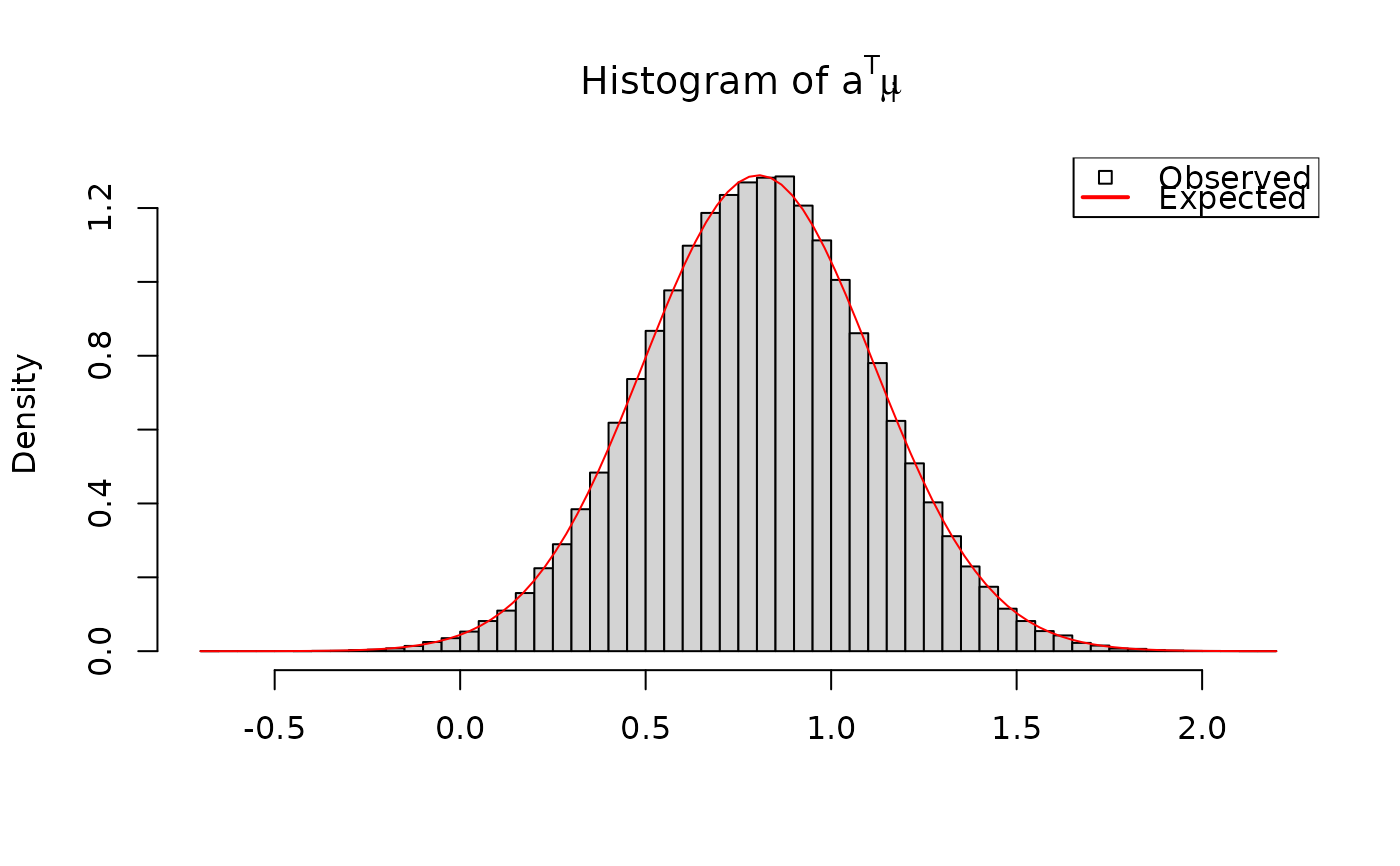
# a' * mu_i is univariate normal with known mean and variance:
a <- rnorm(q) # arbitrary vector
amui <- crossprod(a, out$Mu[iObs,,]) # a' * mu_i
hist(amui, breaks = 100, freq = FALSE,
xlab = "", main = expression("Histogram of "*a^T*mu[i]))
curve(dnorm(x, mean = sum(a * muRx),
sd = sqrt(crossprod(a, SigmaRx %*% a)[1])),
add = TRUE, col = "red")
legend("topright",
legend = c("Observed", "Expected"),
lwd = c(NA, 2), pch = c(22, NA), seg.len = 1.5,
col = c("black", "red"), bg = c("white", NA))
 # sample from p(Beta, Sigma | Mu, Y)
nsamples <- 1e5
out <- RxNormLM(nsamples,
Y = Y, V = V, X = X,
prior = prior,
init = list(Beta = Beta, Sigma = Sigma, Mu = Mu),
burn = floor(nsamples/10),
updateHyp = TRUE,
storeHyp = TRUE,
updateRX = FALSE,
storeRX = FALSE)
# conditional distribution is MNIW:
# calculate the MNIW parameters
OmegaHat <- crossprod(X) + Omega
LambdaHat <- solve(OmegaHat, crossprod(X, Mu) + Omega %*% Lambda)
PsiHat <- Psi + crossprod(Mu) + crossprod(Lambda, Omega %*% Lambda)
PsiHat <- PsiHat - crossprod(LambdaHat, OmegaHat %*% LambdaHat)
nuHat <- nu + n
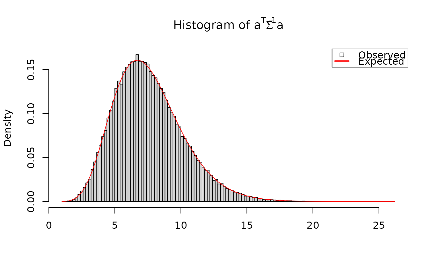
# a' Sigma^{-1} a is chi^2 with known parameters:
a <- rnorm(q)
aSiga <- drop(crossprodV(a, V = out$Sigma, inverse = TRUE))
sigX <- crossprod(a, solve(PsiHat, a))[1]
hist(aSiga, breaks = 100, freq = FALSE,
xlab = "", main = expression("Histogram of "*a^T*Sigma^{-1}*a))
curve(dchisq(x/sigX, df = nuHat)/sigX, add = TRUE, col = "red")
legend("topright",
legend = c("Observed", "Expected"),
lwd = c(NA, 2), pch = c(22, NA), seg.len = 1.5,
col = c("black", "red"), bg = c("white", NA))
# sample from p(Beta, Sigma | Mu, Y)
nsamples <- 1e5
out <- RxNormLM(nsamples,
Y = Y, V = V, X = X,
prior = prior,
init = list(Beta = Beta, Sigma = Sigma, Mu = Mu),
burn = floor(nsamples/10),
updateHyp = TRUE,
storeHyp = TRUE,
updateRX = FALSE,
storeRX = FALSE)
# conditional distribution is MNIW:
# calculate the MNIW parameters
OmegaHat <- crossprod(X) + Omega
LambdaHat <- solve(OmegaHat, crossprod(X, Mu) + Omega %*% Lambda)
PsiHat <- Psi + crossprod(Mu) + crossprod(Lambda, Omega %*% Lambda)
PsiHat <- PsiHat - crossprod(LambdaHat, OmegaHat %*% LambdaHat)
nuHat <- nu + n
# a' Sigma^{-1} a is chi^2 with known parameters:
a <- rnorm(q)
aSiga <- drop(crossprodV(a, V = out$Sigma, inverse = TRUE))
sigX <- crossprod(a, solve(PsiHat, a))[1]
hist(aSiga, breaks = 100, freq = FALSE,
xlab = "", main = expression("Histogram of "*a^T*Sigma^{-1}*a))
curve(dchisq(x/sigX, df = nuHat)/sigX, add = TRUE, col = "red")
legend("topright",
legend = c("Observed", "Expected"),
lwd = c(NA, 2), pch = c(22, NA), seg.len = 1.5,
col = c("black", "red"), bg = c("white", NA))
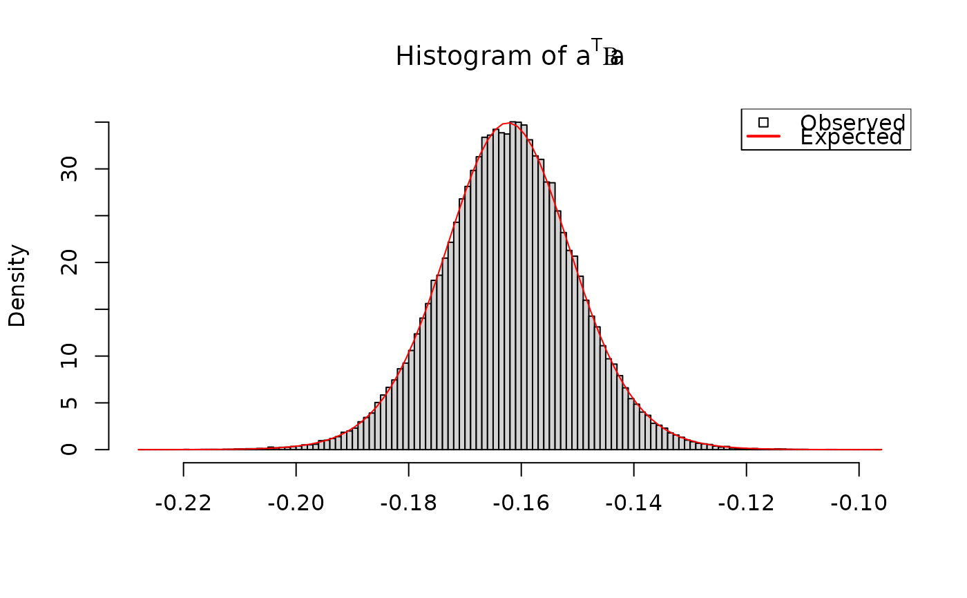
 # a' Beta b is student-t with known parameters:
a <- rnorm(p)
b <- rnorm(q)
# vectorized calculations
aBetab <- crossprodV(X = aperm(out$Beta, c(2,1,3)),
Y = b, V = diag(q)) # Beta b
aBetab <- drop(crossprodV(X = a, Y = aBetab, V = diag(p))) # a' Beta b
# student-t parameters
muT <- crossprod(a, LambdaHat %*% b)[1]
nuT <- nuHat-q+1
sigmaT <- crossprodV(a, V = OmegaHat, inverse = TRUE)[1]
sigmaT <- sigmaT * crossprodV(b, V = PsiHat)[1]
sigmaT <- sqrt(sigmaT / nuT)
hist(aBetab, breaks = 100, freq = FALSE,
xlab = "", main = expression("Histogram of "*a^T*Beta*a))
curve(dt((x-muT)/sigmaT, df = nuT)/sigmaT, add = TRUE, col = "red")
legend("topright",
legend = c("Observed", "Expected"),
lwd = c(NA, 2), pch = c(22, NA), seg.len = 1.5,
col = c("black", "red"), bg = c("white", NA))
# a' Beta b is student-t with known parameters:
a <- rnorm(p)
b <- rnorm(q)
# vectorized calculations
aBetab <- crossprodV(X = aperm(out$Beta, c(2,1,3)),
Y = b, V = diag(q)) # Beta b
aBetab <- drop(crossprodV(X = a, Y = aBetab, V = diag(p))) # a' Beta b
# student-t parameters
muT <- crossprod(a, LambdaHat %*% b)[1]
nuT <- nuHat-q+1
sigmaT <- crossprodV(a, V = OmegaHat, inverse = TRUE)[1]
sigmaT <- sigmaT * crossprodV(b, V = PsiHat)[1]
sigmaT <- sqrt(sigmaT / nuT)
hist(aBetab, breaks = 100, freq = FALSE,
xlab = "", main = expression("Histogram of "*a^T*Beta*a))
curve(dt((x-muT)/sigmaT, df = nuT)/sigmaT, add = TRUE, col = "red")
legend("topright",
legend = c("Observed", "Expected"),
lwd = c(NA, 2), pch = c(22, NA), seg.len = 1.5,
col = c("black", "red"), bg = c("white", NA))