Wishart and Inverse-Wishart distributions.

Densities and random sampling for the Wishart and Inverse-Wishart distributions.

dwish(X, Psi, nu, log = FALSE)

rwish(n, Psi, nu)

diwish(X, Psi, nu, log = FALSE)

riwish(n, Psi, nu)

dwishart(X, Psi, nu, inverse = FALSE, log = FALSE)

rwishart(n, Psi, nu, inverse = FALSE)

Arguments

X: Argument to the density function. Either a q x q matrix or a q x q x n array.
Psi: Scale parameter. Either a q x q matrix or a q x q x n array.
nu: Degrees-of-freedom parameter. A scalar or vector of length n.
log: Logical; whether or not to compute the log-density.
n: Integer number of random samples to generate.
inverse: Logical; whether or not to use the Inverse-Wishart distribution.

Value

A vector length n for density evaluation, or an array of size q x q x n for random sampling.

Details

The Wishart distribution $\boldsymbol{X} \sim \textrm{Wishart}(\boldsymbol{\Psi}, \nu)$ on a symmetric positive-definite random matrix $\boldsymbol{X}$ of size $q \times q$ has PDF $$ f(\boldsymbol{X} \mid \boldsymbol{\Psi}, \nu) = \frac{|\boldsymbol{X}|^{(\nu-q-1)/2}\exp\big\{-\textrm{tr}(\boldsymbol{\Psi}^{-1}\boldsymbol{X})/2\big\}}{2^{q\nu/2}|\boldsymbol{\Psi}|^{\nu/2} \Gamma_q(\frac \nu 2)}, $$ where $\Gamma_q(\alpha)$ is the multivariate gamma function, $$ \Gamma_q(\alpha) = \pi^{q(q-1)/4} \prod_{i=1}^q \Gamma(\alpha + (1-i)/2). $$ The Inverse-Wishart distribution $\boldsymbol{X} \sim \textrm{Inverse-Wishart}(\boldsymbol{\Psi}, \nu)$ is defined as $\boldsymbol{X}^{-1} \sim \textrm{Wishart}(\boldsymbol{\Psi}^{-1}, \nu)$.

dwish() and diwish() are convenience wrappers for dwishart(), and similarly rwish() and riwish() are wrappers for rwishart().

Examples

# Random sampling

n <- 1e5
q <- 3
Psi1 <- crossprod(matrix(rnorm(q^2),q,q))
nu <- q + runif(1, 0, 5)

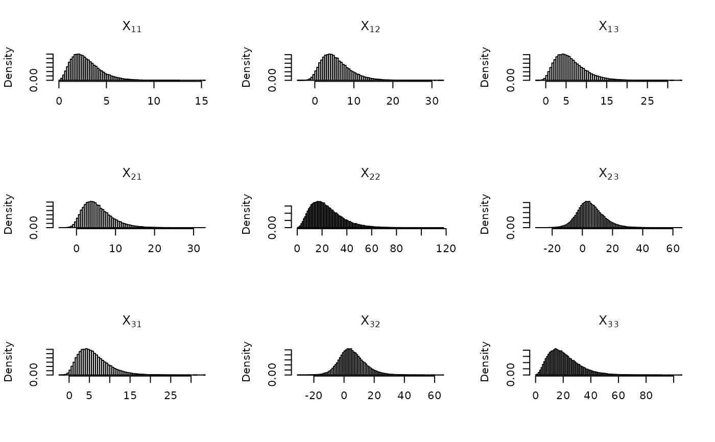
X1 <- rwish(n,Psi1,nu) # Wishart

# plot it
plot_fun <- function(X) {
  q <- dim(X)[1]
  par(mfrow = c(q,q))
  for(ii in 1:q) {
    for(jj in 1:q) {
      hist(X[ii,jj,], breaks = 100, freq = FALSE,
           xlab = "", main = parse(text = paste0("X[", ii, jj, "]")))
    }
  }
}

plot_fun(X1)


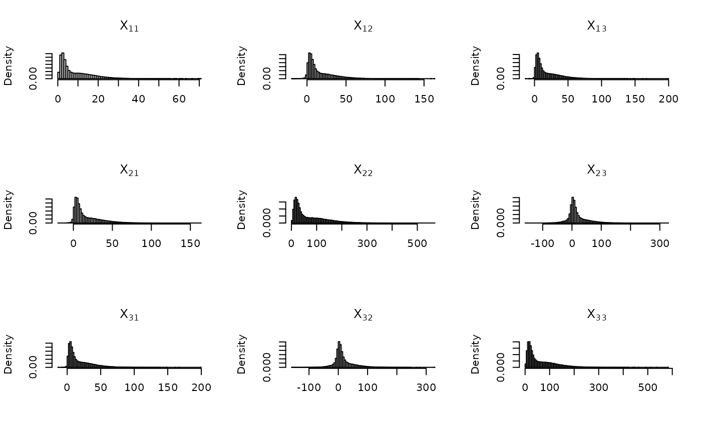
# "vectorized" scale parameeter
Psi2 <- 5 * Psi1
vPsi <- array(c(Psi1, Psi2), dim = c(q, q, n))
X2 <- rwish(n, Psi = vPsi, nu = nu)
plot_fun(X2)


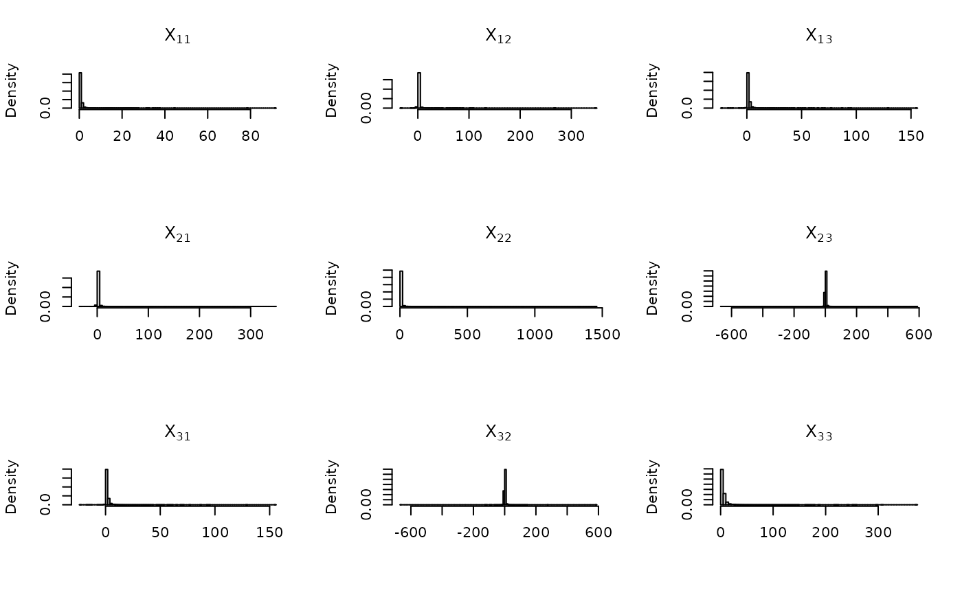
# Inverse-Wishart
X3 <- riwish(n, Psi2, nu)
plot_fun(X3)


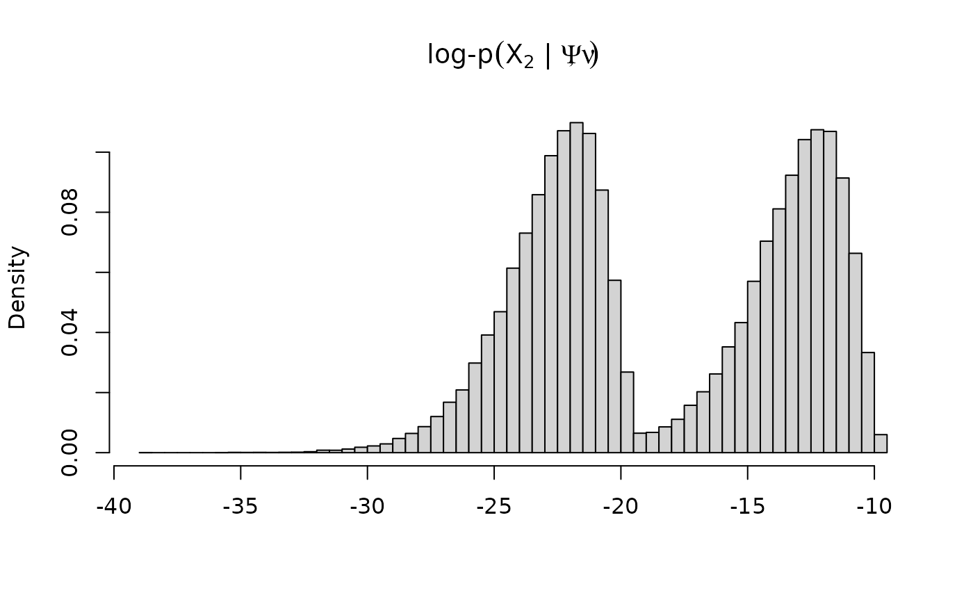
# log-density calculation for sampled values
par(mfrow = c(1,1))
hist(dwish(X2, vPsi, nu, log = TRUE),
     breaks = 100, freq = FALSE, xlab = "",
     main = expression("log-p"*(X[2]*" | "*list(Psi,nu))))